Keyboard shortcuts

Press ← or → to navigate between chapters

Press S or / to search in the book

Press ? to show this help

Press Esc to hide this help

Open-source · full-custom IC design

From schematic to sign-off,
in one native app.

IC Studio puts schematic capture, SPICE simulation, layout, automatic place and route, DRC, LVS and parasitic extraction on one design database. Draw a circuit, generate its layout, verify it and simulate it again with the parasitics, without leaving the window or converting a single file.
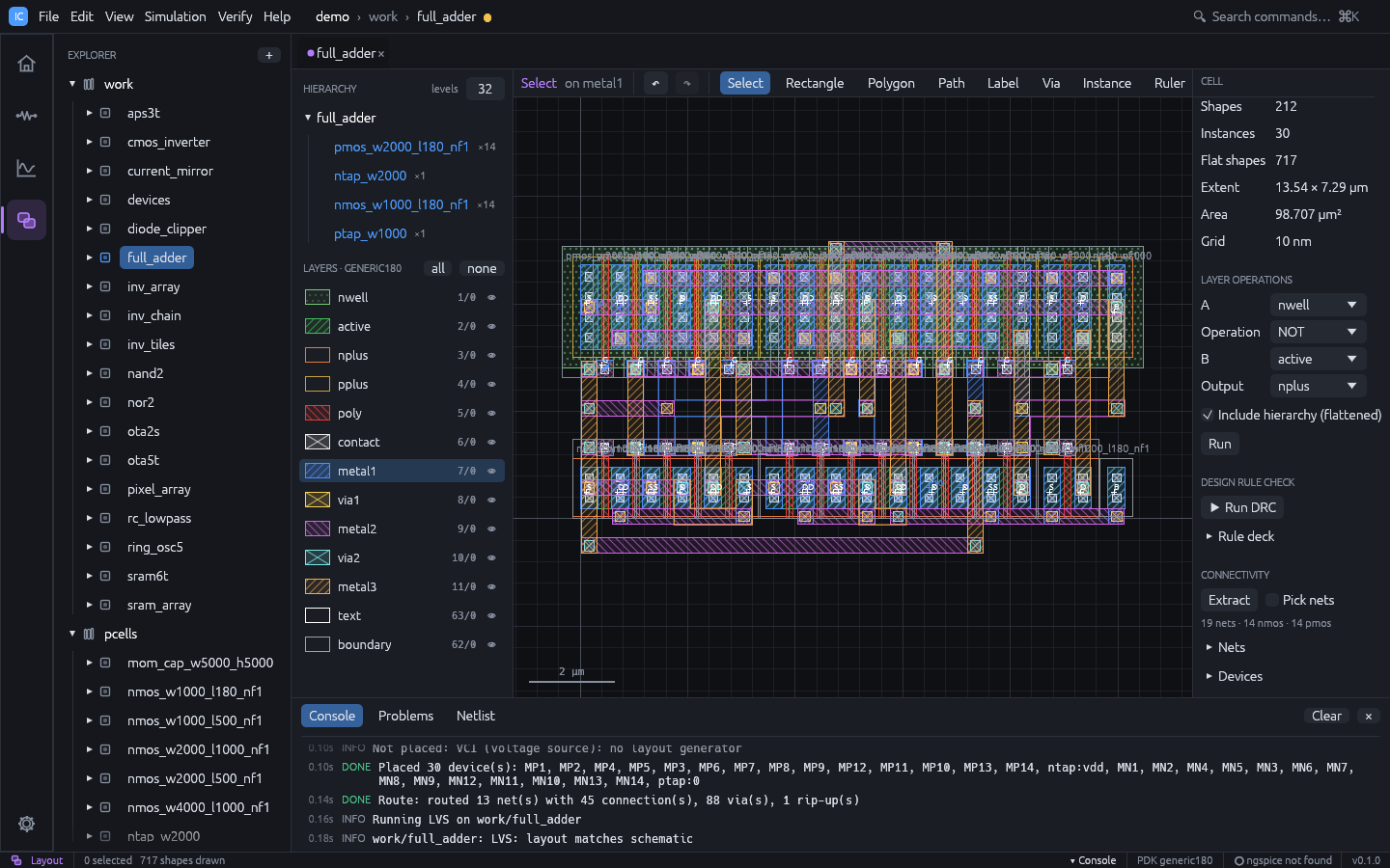
Auto place and route: a 28-transistor full adder generated from its schematic, LVS clean

28Tfull adder placed and routed automatically, DRC and LVS clean
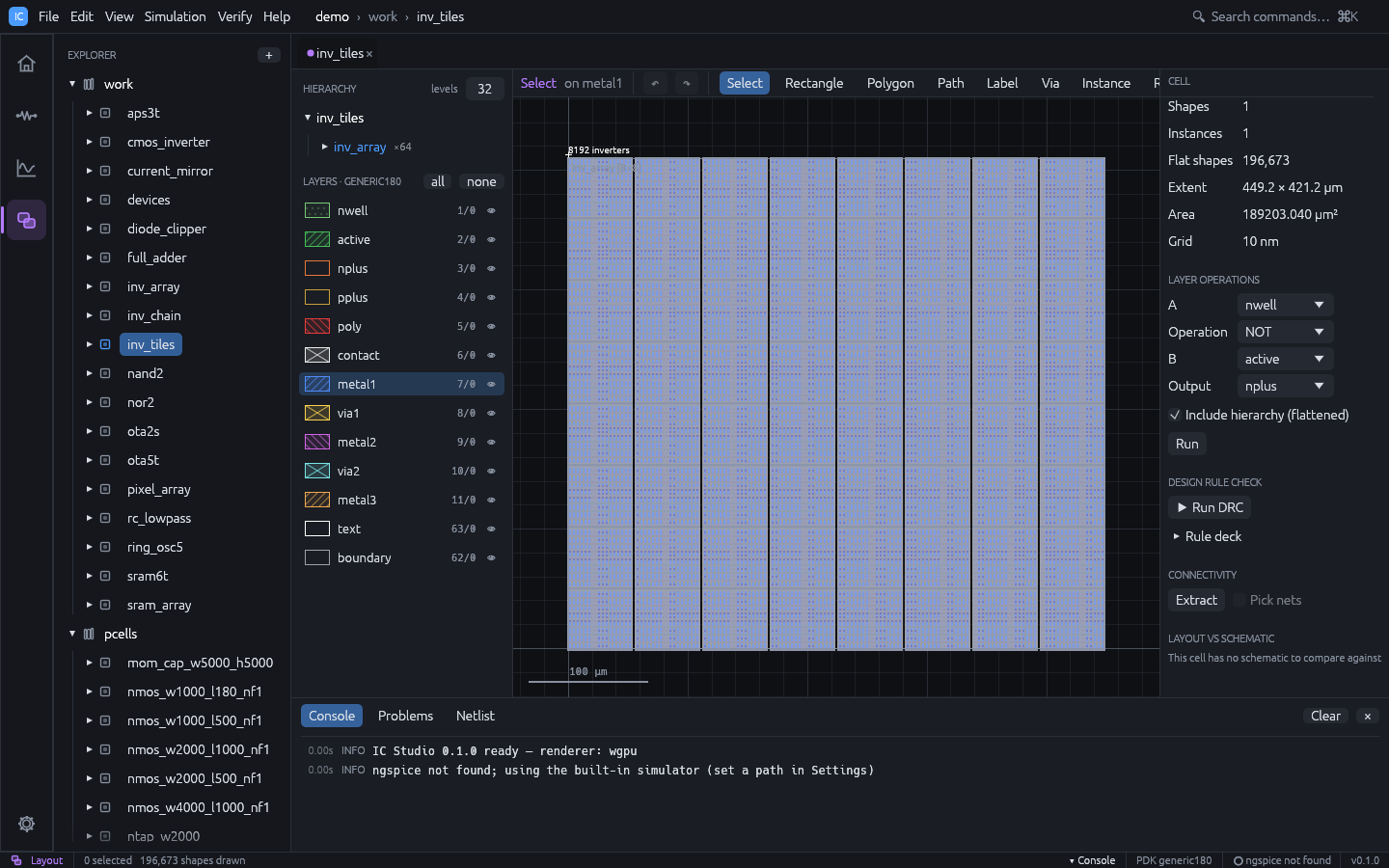
8,192inverters (about 250k shapes) browsed interactively
3front ends on one core: desktop app, CLI, MCP for AI agents
3 OSWindows, Linux and macOS, GPU rendered with wgpu

One database, the whole loop

Most open-source flows chain separate tools through netlists and GDS files. In IC Studio the schematic, the simulator and the layout share one design database, so every step knows about the others:

Schematic→ Simulate→ Generate layout→ Route→ DRC · LVS→ Extract parasitics→ Simulate again ↺
  • Layouts are generated from schematics and routed automatically.
  • Layouts are checked against schematics (LVS) with clickable differences.
  • Parasitics extracted from the layout flow straight back into simulation.

What you get

SCH

Schematic and simulation

Live connectivity, operating-point annotation, DC / AC / transient analyses on a built-in simulator or ngspice, Bode plots and automatic measurements.

P&R

Automatic place and route

Transistors placed as PCells with shared diffusion, common-centroid matching and dummies; a rip-up-and-reroute maze router wires every net DRC-clean.

LAY

Hierarchical layout

Instances and arrays, level-of-detail rendering for large designs, Boolean layer operations, vias, PCells, GDSII and OASIS in and out.

DRC

Verification

Rule-deck DRC with derived layers, connectivity extraction, LVS with device merging, and sign-off runs through KLayout, Calibre or netgen.

ADE

Analysis tools

A waveform calculator, corner, parametric and Monte Carlo sweeps with specs, yield and datasheets, and run-to-run comparison of results.

GEN

Layout generators

Guard rings, via arrays, common-centroid matched placement and density fill, plus a visual DRC rule designer and Virtuoso-compatible SKILL.

PDK

Real PDKs

Start on the generic 180 nm technology, then switch to SKY130 or IHP SG13G2: layers, device recognition, models and corners from one PDK file.

AI

Scriptable and agent-ready

Every action is a command. The ics CLI runs in CI, and the MCP server lets an AI agent design in the window you are watching.

Try it in one minute

git clone https://github.com/geniuskey/ic-studio
cd ic-studio
cargo run --release -- --demo --cell full_adder --workspace layout

With a release installed, run ic-studio --demo --cell full_adder --workspace layout instead. The demo project opens on an automatically placed and routed full adder. The demo gallery walks through every example and has ready-made scripts for presenting IC Studio live.

What is in the box

Two programs, installed together:

ProgramPurpose
ic-studioThe desktop application
icsCommand-line interface for scripting and CI
ics mcpThe same ics program run as a Model Context Protocol server for AI agents

All three front ends use the same core library, so a project edited in the app can be simulated, checked or exported from the command line, or driven by an agent.

Main concepts

  • Project: a folder holding ic-studio.json, the technology (tech.json) and one folder per library. Everything is human-readable JSON that diffs well in git.
  • Library: a named group of cells (the demo project has work and pcells).
  • Cell: a design unit with up to three views: schematic, simulation (the analyses set up for the schematic) and layout.
  • Workspace: the app has four workspaces, Home, Schematic, Simulation and Layout. The open cells appear as tabs shared by all workspaces; switching workspace shows the same cell in a different view.
  • Technology (PDK): layers, GDS numbers, display styles, design rules and electrical coefficients. New projects start with a generic 180 nm-class technology.

How to read this guide

Keyboard shortcuts are written for Windows and Linux (Ctrl). On macOS use Cmd instead. Press F1 in the app for the full shortcut list, or see Keyboard shortcuts.

Installation

Install a release build with one command, or build IC Studio from source with the Rust toolchain.

Install a release

Windows (PowerShell):

irm https://github.com/geniuskey/ic-studio/releases/latest/download/install.ps1 | iex

macOS (Apple silicon) and Linux (x86_64):

curl -fsSL https://github.com/geniuskey/ic-studio/releases/latest/download/install.sh | sh

The installer downloads the latest release and installs two programs into one folder: the desktop app ic-studio and the command line tool ics, which is also the MCP server for AI agents (ics mcp).

WindowsmacOS / Linux
Folder%LOCALAPPDATA%\Programs\IC Studio~/.local/share/ic-studio
On the PATHfolder added to the user PATHlinks in ~/.local/bin
LauncherStart Menu shortcut IC Studio~/.local/share/applications/ic-studio.desktop (Linux)

The installer also:

  • registers the MCP server with Claude Code if claude is on the PATH (claude mcp add --scope user ic-studio -- <folder>/ics mcp); otherwise it prints that command and the JSON config for other clients (see MCP server);
  • on macOS, removes the download quarantine attribute;
  • on macOS / Linux, prints the line to add to your shell profile if ~/.local/bin is not on the PATH. On Windows, open a new terminal to pick up the PATH change.

To update, run the installer again; this works while the app or an agent is running (restart them afterwards). The app’s own updater (Help > Check for Updates…) also replaces ics together with the app.

Options are environment variables:

VariableEffect
ICS_VERSIONInstall this release tag, e.g. v0.2.0 (default: latest)
ICS_INSTALL_DIRInstall into this folder
ICS_UNINSTALL=1Remove the folder, the PATH entry or links, the launcher and the MCP registration
$env:ICS_VERSION="v0.2.0"; irm https://github.com/geniuskey/ic-studio/releases/latest/download/install.ps1 | iex
curl -fsSL https://github.com/geniuskey/ic-studio/releases/latest/download/install.sh | ICS_UNINSTALL=1 sh

Release builds exist for Windows x86_64, Linux x86_64 and macOS on Apple silicon. On an Intel Mac, build from source.

Manual download. Each release has an archive with both programs, ic-studio-<platform>.zip (Windows) or ic-studio-<platform>.tar.gz (macOS, Linux), where <platform> is windows-x86_64, linux-x86_64 or macos-aarch64. Unpack it into a folder of your choice and keep the two programs together: the updater and Add to Claude Code look for ics next to ic-studio. Put the folder on the PATH to use ics in a terminal.

Build from source

Requirements

  • Rust 1.95 or newer from rustup.rs.
  • Windows: the MSVC toolchain (x86_64-pc-windows-msvc), which needs the Visual Studio Build Tools with the “Desktop development with C++” workload.
  • Linux: the windowing libraries libxkbcommon-dev libwayland-dev libx11-dev libxcursor-dev libxrandr-dev libxi-dev.
  • macOS: the Xcode command line tools.
  • A GPU driver supported by wgpu (DX12 on Windows, Vulkan on Linux, Metal on macOS).

Build and run

git clone https://github.com/geniuskey/ic-studio
cd ic-studio
cargo run --release                     # the desktop app
cargo run --release -- --demo           # with the bundled demo designs
cargo run --release -- path/to/project  # open a project folder

To build both programs (ic-studio, ics) into target/release/:

cargo build --release --workspace

Launch options

ic-studio [PROJECT_DIR] [--demo] [--cell NAME] [--workspace home|schematic|simulation|layout] [--run]
OptionEffect
PROJECT_DIROpen this project folder
--demoOpen the demo project (in memory, not saved until you save it)
--cell NAME, -c NAMEOpen the cell with this name
--workspace W, -w WStart in this workspace
--runRun the cell’s simulation on startup

Example: cargo run --release -- --demo --cell inv_tiles --workspace layout.

Without arguments, the app reopens the most recent project if Reopen last project is checked in Settings (the default), otherwise it shows the welcome page.

ngspice (optional)

IC Studio has its own built-in simulator, so ngspice is not required. To use ngspice as a backend, install it:

  • Windows: the official build, which installs to C:\Spice64\bin\
  • macOS: brew install ngspice
  • Linux: apt install ngspice (or your distribution’s package)

IC Studio looks for /opt/homebrew/bin/ngspice, /usr/local/bin/ngspice, /usr/bin/ngspice and C:\Spice64\bin\ngspice.exe, then for ngspice on the PATH. To use another location, open File > Settings… (Ctrl+,), enter the path in the ngspice field and press Detect. The status bar and the console show whether ngspice was found.

On Windows, ngspice.exe is the GUI build; if detection or batch simulation fails, point the setting at the console binary ngspice_con.exe in the same folder.

Settings

File > Settings… (Ctrl+,, also in the Tools menu, or the gear at the bottom of the activity bar):

SettingMeaning
ThemeDark or Light (also View > Light Theme / Dark Theme)
UI scale0.75 to 1.75
ngspicePath to the ngspice executable, with Detect
InteractionMouse profile: Virtuoso (default) or Conventional (see Keyboard shortcuts)
StartupReopen last project; Check for updates on startup
AIAI Models…: provider, model and API key of the Design Copilot
AI agents (MCP)Add to Claude Code registers ics mcp with Claude Code; Copy MCP config copies the JSON for other clients (see MCP server)

Settings and the recent-projects list are stored by the app between sessions.

Example projects with real PDKs

Scripts download open-source designs into examples/ (git-ignored) as ready-to-open projects:

./scripts/fetch-examples.sh             # macOS / Linux (curl, gunzip)
./scripts/fetch-examples.ps1            # Windows PowerShell
#   --caravel / -Caravel  also the full caravel chip (52 MB download, 278 MB unpacked)
#   --force   / -Force    rebuild the projects from the downloaded files
  • examples/sky130: SKY130 layer set with the efabless caravel libraries caravel_clocking, housekeeping and chip_io (and caravel).
  • examples/gf180: GF180MCU layer set with the gf180mcu_fd_sc_mcu7t5v0 standard cells and the gf180mcu_fd_ip_sram 512 x 8 SRAM macro.

Open them with File > Open Project… or ic-studio examples/sky130.

Quick tour

This tour walks through the demo project: simulation, hierarchical layout, automatic place and route, verification and post-layout simulation. It ends by building a small circuit from scratch.

Open the demo project

cargo run --release -- --demo

Or choose Open demo project on the welcome page (File > New Demo Project). The demo lives in memory until you save it with Ctrl+S. All cells are in the work library and use the generic 180 nm technology.

The demo gallery describes every cell, and has scripts for presenting IC Studio to others.

The pcells library holds the PCell variants the layouts use.

1. Schematic and simulation

  1. In the Explorer, click cmos_inverter. The schematic opens.
  2. Press F5. The Simulation workspace opens with the DC sweep and transient results.
  3. Tick or untick signals in Signals to change the plot; read MIN / MAX / FINAL in Measurements.
  4. Press Ctrl+2 to go back to the schematic: node voltages and drain currents from the operating point are annotated on it.
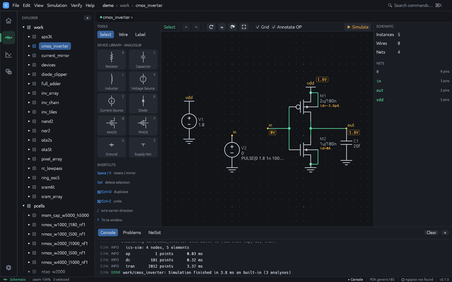
Schematic with OP annotation

Try rc_lowpass (AC: the f -3 dB column shows the corner frequency) and ota5t (AC: open-loop gain and unity-gain frequency).

2. Layout and hierarchy

  1. Press Ctrl+4 with cmos_inverter open. This layout was drawn by hand.
  2. Open inv_tiles (Explorer, or Ctrl+K and type inv_tiles). Zoom with Ctrl+wheel, pan with the wheel or the middle mouse button, and press F to fit.
  3. Press 1, 2 and 9 to change how many hierarchy levels are drawn.
  4. Double-click an instance to open the placed cell.

3. Automatic place and route

  1. Open full_adder and press Ctrl+4. This layout was not drawn: it was generated from the schematic and routed automatically.
  2. Press Ctrl+A and Delete to clear it.
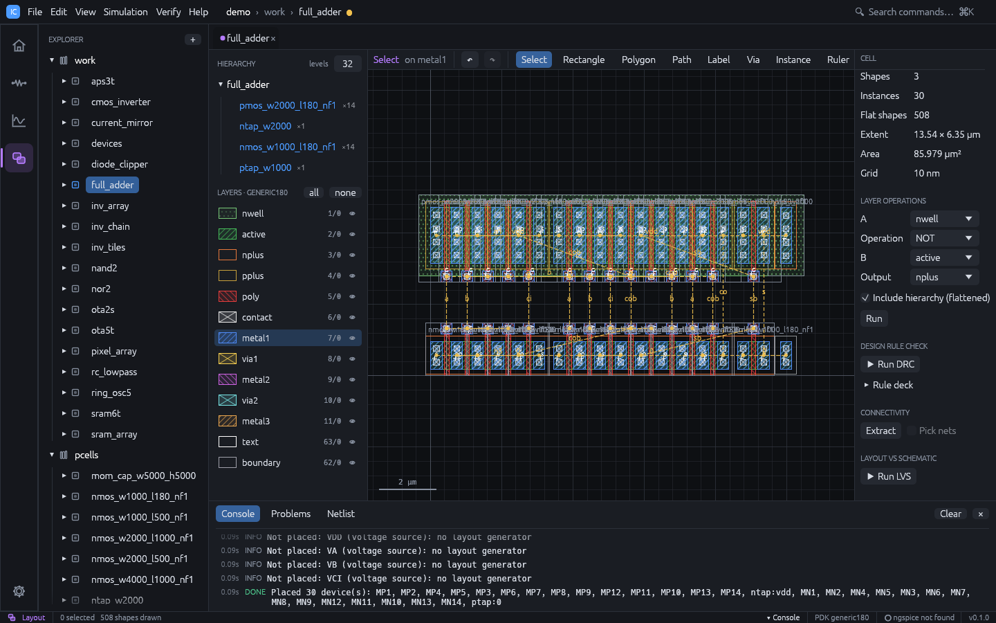
  3. Choose Verify > Generate Layout from Schematic. The 28 transistors are placed and flylines show the connections to make.
  4. Choose Verify > Route Flylines. Every net is routed on metal.

Generated and routed full adder

4. Verification

  1. Open nand2 and switch to the Layout workspace.
  2. In the right panel, press Run DRC: no violations.
  3. Press Run LVS: the layout matches the schematic.
  4. Open cmos_inverter and run LVS: it lists the deliberate differences. Click one to zoom to it.
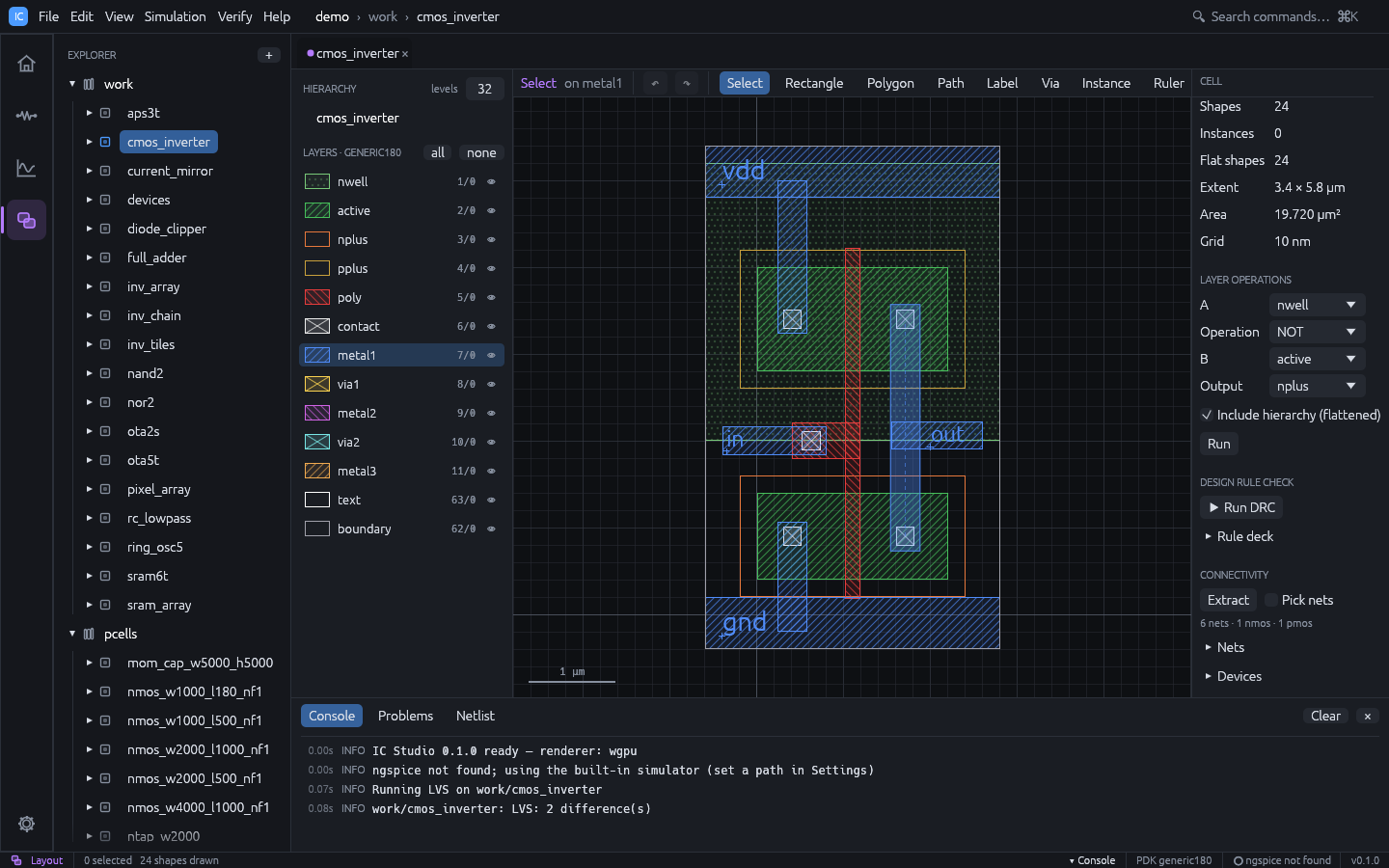
LVS result

5. Post-layout simulation

  1. Open ring_osc5 in the Simulation workspace.
  2. Press F5 and note the oscillation period in the transient plot.
  3. Tick Include layout parasitics and press F5 again. The console summarises the extracted capacitance and resistance. Compare the period: the added wire capacitance and resistance slow the oscillator down.

6. Build an inverter from scratch

  1. Press Ctrl+N, name the cell my_inv, keep schematic checked, and press Create.
  2. Press P and click to place a PMOS, then press N and click below it to place an NMOS. Press Esc.
  3. Press W and wire the two drains together, then the two gates. Esc ends a wire.
  4. Press S and place a supply symbol on the PMOS source; press G and place ground on the NMOS source. Wire them.
  5. Press T, type in in the Net: field and click on the gate wire; type out and click on the drain wire.
  6. Add the sources: press V, place a source, wire its p pin to the supply net and its n pin to a ground symbol; set DC value to 1.8 in the inspector. Place a second source for in with Transient PULSE(0 1.8 1n 100p 100p 2n 4n).
  7. Press Ctrl+3, enable Transient (step 10p, stop 10n) and press F5.
  8. Choose Verify > Generate Layout from Schematic. The two transistors are placed as PCells with well taps, and flylines show the connections to make.
  9. Choose Verify > Route Flylines. The router wires the nets on metal.
  10. Run DRC and LVS from the right panel, then save with Ctrl+S.

See Schematic-driven layout for what the generator and the router do, and how to match devices.

7. Command line

The same project can be checked from a terminal:

ics new demo --template demo
ics sim demo ota5t
ics drc demo nand2
ics lvs demo nand2

See Command line.

Demo gallery

Every example below ships with IC Studio. Open them all with:

cargo run --release -- --demo

or choose Open demo project on the welcome page. The demo uses the generic 180 nm technology and lives in memory until you save it with Ctrl+S. To jump straight to a cell, add --cell <name> --workspace <schematic|simulation|layout>.

The second half of this page has step-by-step demo scripts for showing IC Studio to an audience.

Highlights

All demo cells

CellWhat it shows
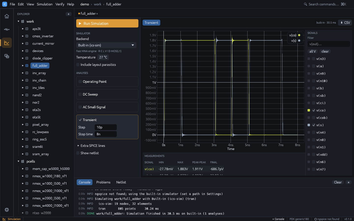
full_adder28T mirror full adder, placed and routed automatically; transient over all input combinations
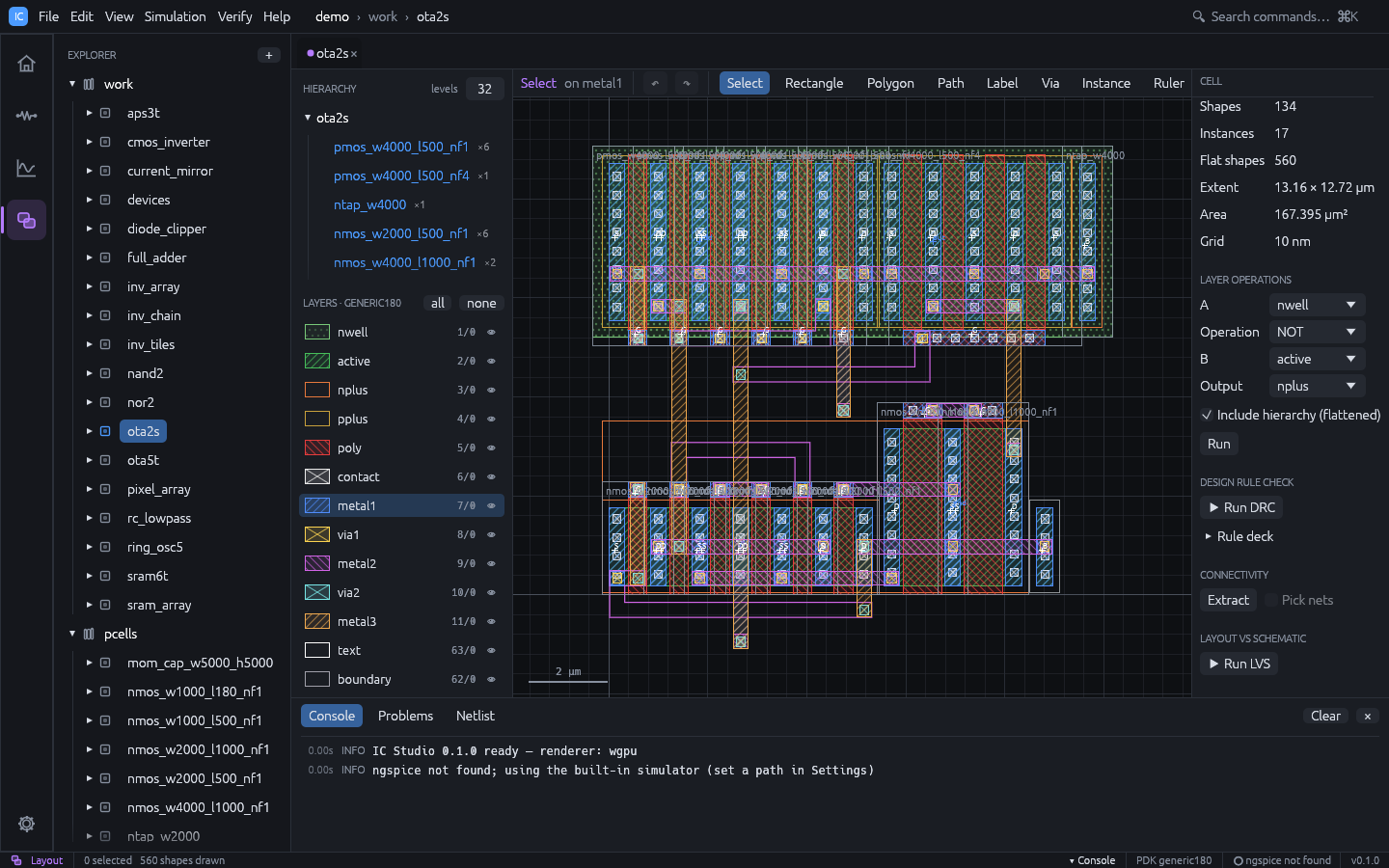
ota2sTwo-stage OTA, auto P&R with common-centroid matching; about 80 dB open-loop gain in AC
cmos_inverterInverter with a hand-drawn layout; LVS reports deliberate findings (PMOS W, load cap)
rc_lowpassRC low-pass filter (fc about 159 kHz): OP, AC and transient
diode_clipperResistor and shunt diode clipper: transient and DC sweep
nand22-input NAND: schematic plus routed PCell layout, DRC and LVS clean
nor22-input NOR: schematic plus routed PCell layout, DRC and LVS clean
ring_osc55-stage ring oscillator, fully routed; slows down visibly with layout parasitics
current_mirrorNMOS current mirror with a 20 µA reference: DC sweep of the output
ota5t5-transistor OTA: about 42 dB open-loop gain in AC
sram6t6T SRAM bit cell, DRC and LVS clean: transient write and hold
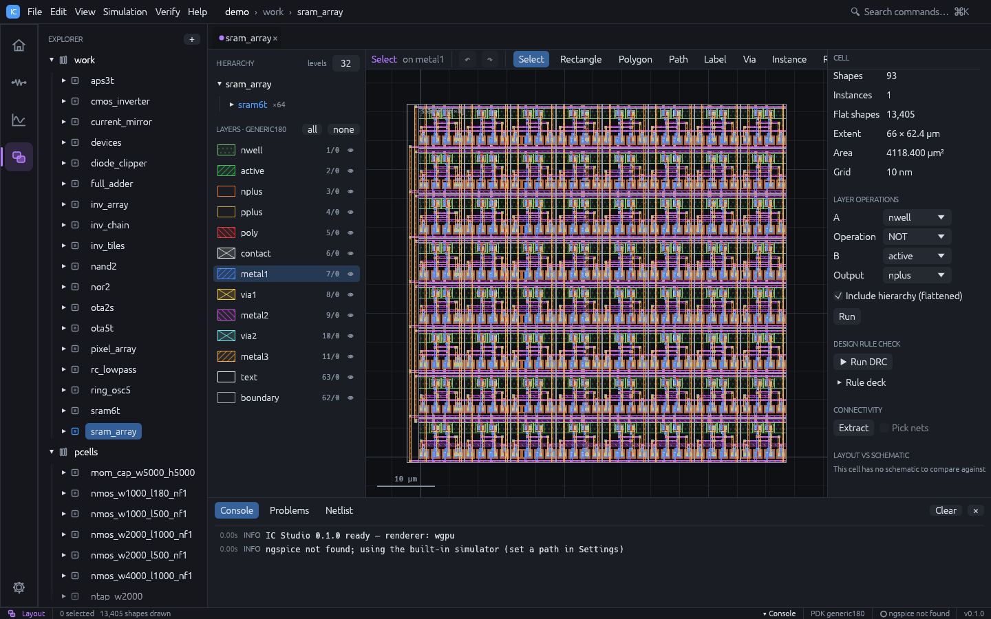
sram_array8 × 8 array of sram6t
aps3t3T image sensor pixel, DRC and LVS clean: transient reset and integration
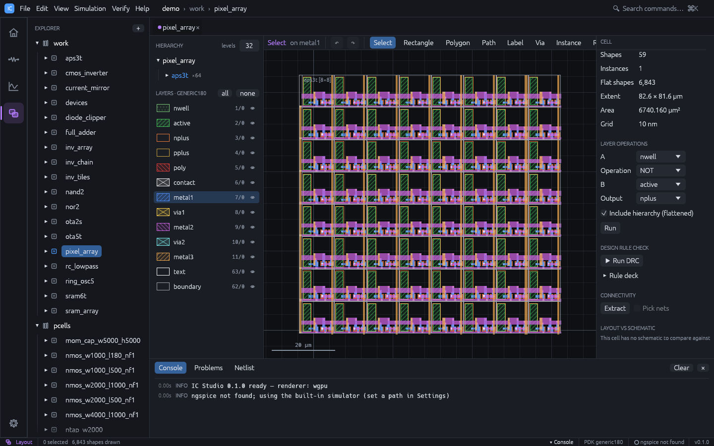
pixel_array8 × 8 array of aps3t
inv_chainFour placed cmos_inverter instances
inv_array16 × 8 array of inverters
inv_tiles8 × 8 array of inv_array: 8,192 inverters, two levels of hierarchy
devicesOne instance of every PCell

Every cell with both a schematic and a layout (full_adder, ota2s, nand2, nor2, ring_osc5, current_mirror, ota5t, sram6t, aps3t) runs the whole flow: simulate, open the layout, run DRC and LVS, and simulate again with parasitics.

Demo scripts

Each script is a sequence you can run in front of an audience, with the result to expect at every step. The blue boxes suggest what to say.

1. Five-minute tour

The whole loop on one circuit: schematic, simulation, automatic layout, verification and post-layout simulation.

  1. Start the app on the adder’s schematic:

    cargo run --release -- --demo --cell full_adder --workspace schematic
    
  2. Press F5. The Simulation workspace opens with the transient run: a, b and ci step through all eight combinations, and s and co follow the truth table.

  3. Press Ctrl+4 for the layout. Select everything with Ctrl+A and press Delete. The layout is empty.

  4. Choose Verify > Generate Layout from Schematic. The 28 transistors appear as PCells in a PMOS row over an NMOS row, with well taps, and dashed flylines show every connection still to make.

  5. Choose Verify > Route Flylines. The flylines are replaced by metal1 to metal3 wires and vias; the console reports the nets routed.

  6. In the right panel press Run DRC (no violations), then Run LVS (the layout matches the schematic).

  7. Press Ctrl+3, tick Include layout parasitics and press F5. The console summarises the extracted capacitance and resistance, and the waveforms now include the wiring delay.

Say: “Nothing here was drawn by hand. The layout comes from the schematic, the router makes it DRC clean, LVS proves it is the same circuit, and the parasitics go straight back into the simulation, all on one database.”

2. Auto place and route, step by step

Slower, for an audience that cares about layout. Use the adder or the OTA.

StepDoExpect
1Open full_adder in the Layout workspaceThe finished, routed layout
2Ctrl+A, DeleteAn empty layout
3Verify > Generate Layout from SchematicDevices placed; source / drain columns shared where nets allow; flylines on
4Move a device with the mouseIts flylines follow it: the link to the schematic is the instance name
5Ctrl+ZThe device goes back
6Verify > Route FlylinesAll nets routed; the console lists nets, connections, vias and rip-ups
7Click a device in the layout, then Ctrl+2The same device is selected in the schematic (cross-probing)
8Run DRC, Run LVSNo violations; layout matches schematic

Placement with flylines, before routing

Say: “The router is a maze router with rip-up and reroute. Its grid is aligned to the device terminals, so what it draws is DRC clean by construction, and it labels the named nets so LVS can anchor them.”

3. Analog matching

Shows that the generator understands analog structure, not only connectivity.

  1. Open ota2s in the Layout workspace, Ctrl+A, Delete.
  2. Verify > Generate Layout from Schematic. The console reports the matched groups, for example the differential pair and the mirror placed as ABBA with dummy fingers at both ends.
  3. Verify > Route Flylines, then Run LVS. LVS merges the unit fingers back into the seven schematic devices and ignores the dummies.
  4. Press Ctrl+3 and F5. The AC plot shows about 80 dB of open-loop gain.

Say: “Differential pairs and current mirrors are detected from the schematic. They are split into unit fingers and placed in common-centroid order, the way an analog layout engineer would, and LVS still sees seven transistors.”

4. Post-layout effects

  1. Open ring_osc5 in the Simulation workspace and press F5. Note the oscillation period.
  2. Tick Include layout parasitics and press F5 again. The period gets longer: the wire capacitance and resistance extracted from the layout slow the ring down.

5. Scale

  1. Open inv_tiles in the Layout workspace: 8,192 inverters.
  2. Zoom with Ctrl+wheel, pan with the wheel or the middle mouse button, F to fit.
  3. Press 1, 2 and 9 to change how many hierarchy levels are drawn, and double-click an instance to descend into it.

6. Command line and CI

The same flow without a window, from a SPICE netlist to a verified GDS. Save this as ota.cir:

* two-stage OTA
M1 x inp tail 0 nmos w=4u l=500n
M2 o1 inn tail 0 nmos w=4u l=500n
M3 x x vdd vdd pmos w=8u l=500n
M4 o1 x vdd vdd pmos w=8u l=500n
M5 tail vb 0 0 nmos w=4u l=1u
M6 out o1 vdd vdd pmos w=16u l=500n
M7 out vb 0 0 nmos w=4u l=1u
VDD vdd 0 dc 1.8
VINP inp 0 dc 0.9 ac 1
VINN inn 0 dc 0.9
VB vb 0 dc 0.65
.ac dec 20 1k 10g

Then:

ics new demo                         # project with the demo cells
ics schematic demo my_ota ota.cir    # netlist -> schematic and simulation setup
ics route demo my_ota --place        # place, route, save
ics drc demo my_ota                  # 0 violations
ics lvs demo my_ota                  # layout matches schematic
ics sim demo my_ota --parasitics     # post-layout AC
ics gds demo my_ota -o my_ota.gds    # stream out

Every command exits non-zero on failure, so the sequence drops into a CI job as is. See Command line.

7. An AI agent designs while you watch

With the MCP server registered in an agent such as Claude Code, start the app (cargo run --release -- --demo) and ask the agent:

In the open IC Studio project, create a cell my_ota from this netlist (paste ota.cir), generate its layout, route it, run DRC and LVS, then simulate AC and tell me the open-loop gain.

The status bar shows MCP live. The schematic appears in the window, then the placed devices, the routed wires, the DRC and LVS results and the AC plot, each logged in the console as MCP · <tool> .... Every layout step can be undone with Ctrl+Z.
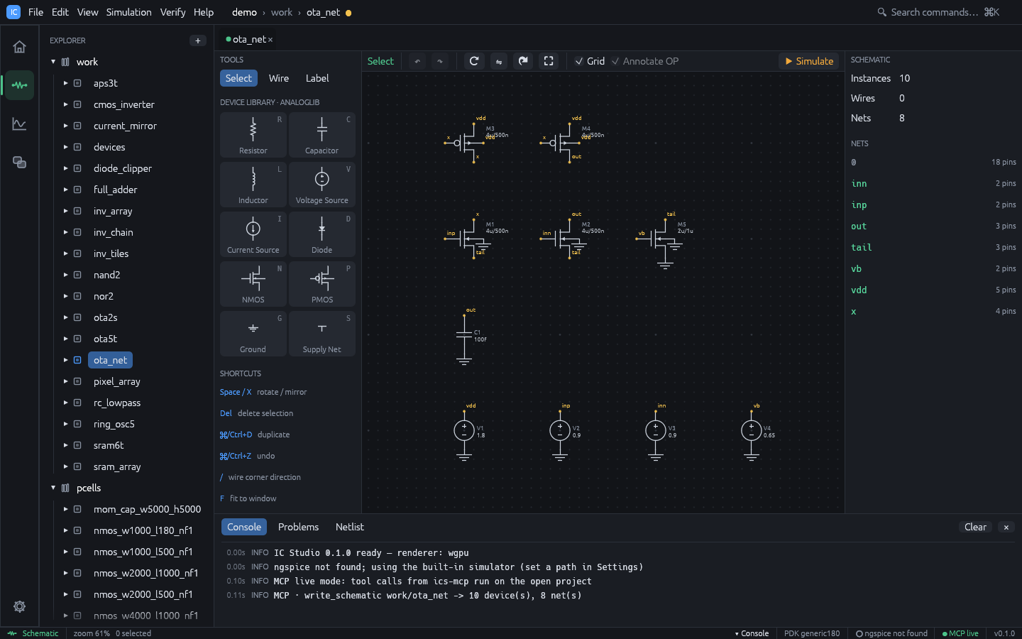
An agent writing a schematic in live mode

Say: “The agent uses the same commands as the menus. It is not generating a file for you to import; it is working in your session, and you can take over at any point.”

Projects, libraries and cells

The window
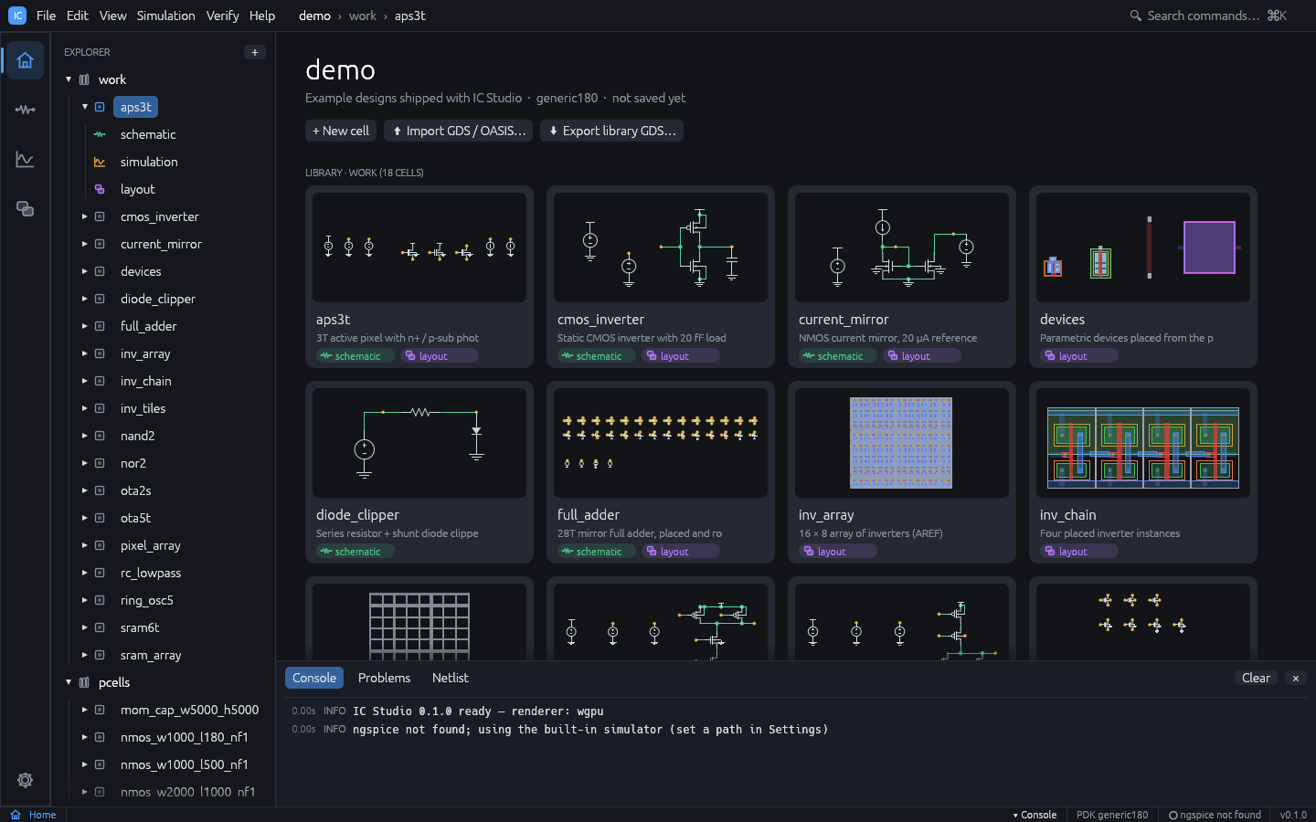
Project home

  • Menu bar (see Menus below) with a breadcrumb project > library > cell. A dot after the cell name means unsaved changes. On the right, Search commands… opens the command palette.
  • Activity bar (far left): the four workspaces Home, Schematic, Simulation and Layout (Ctrl+1 to Ctrl+4), and the Settings gear at the bottom.
  • Explorer: libraries, cells and their views.
  • Cell tabs above the editor. Ctrl+W closes the active tab.
  • Bottom panel (Ctrl+J): Console (log), CIW (SKILL prompt), Problems (schematic checker findings) and Netlist (the SPICE netlist of the active cell).
  • Menus: File, Edit, View, Simulation, Verify, Tools (design copilot, optimizer, calculator, sweeps, results and browsers, generators, DRC rule designer, stream layer map, dummy fill, SKILL; see Tools) and Help (user guide, shortcuts, check for updates). In the Layout workspace the Create and Options menus are added.
  • Status bar: workspace, zoom, selection, technology name, ngspice status and, while an agent is connected, “MCP live”.

Creating and opening projects

The welcome page (shown when no project is open) has three cards: Open demo project, New project… and Open project…, plus a list of recent projects.

  • File > New Project…: enter a name (letters, digits, _ and -) and a parent folder. The project is created in <folder>/<name> with the generic 180 nm technology. Check the demo option to start from the demo designs instead.
  • File > New Demo Project: creates the demo project in memory. Use File > Save to choose a folder.
  • File > Open Project… (Ctrl+O): pick the project folder (the one containing ic-studio.json). File > Open Recent lists recent projects.
  • File > Save (Ctrl+S) and Save As… (Ctrl+Shift+S). When saving to a folder that is neither empty nor an existing project, a subfolder named after the project is created.
  • File > Close Project. Closing, quitting or opening another project with unsaved changes asks whether to Save, Discard or Cancel.

Cells and views

  • New cell (Ctrl+N, the + in the Explorer header or + New cell on the Home page): choose the library, a cell name, an optional description and which views to create (schematic, layout).
  • Click a cell in the Explorer to open it. Expand it to see its schematic, simulation and layout views; a missing view is shown dimmed with + create, and clicking it creates an empty view.
  • Right-click a cell for Open schematic, Open layout, Rename… and Delete…. Deleting removes the cell’s files from disk when the project is saved.
  • The Home workspace shows the project overview: a thumbnail card per cell, plus + New cell, Import GDS / OASIS… and Export library GDS… buttons.

Command palette

Ctrl+K or Ctrl+Shift+P opens the palette. Type words to filter (all words must match), use the arrow keys and Enter to run a command, Esc to close. It contains every menu action plus Open <lib>/<cell> · schematic and · layout entries for every cell, which makes it the fastest way to jump between cells.

On-disk format

A project is a folder of plain JSON files that work well with version control:

myproj/
  ic-studio.json          project manifest
  tech.json               technology: layers, rules, DRC deck, coefficients
  work/                   one folder per library
    cmos_inverter/        one folder per cell
      cell.json           cell metadata (name, description)
      schematic.json      schematic view (if present)
      layout.json         layout view (if present)
      sim.json            simulation setup

Libraries imported from GDS are stored differently (as a GDS file in the library folder with a library.json), so large imports stay compact.

Import and export

ActionMenu
Import a GDSII or OASIS file as a new libraryFile > Import > GDSII / OASIS…
Import a KLayout layer properties file as the technologyFile > Import > KLayout layer properties…
Replace the technology with a PDK fileFile > Import > PDK…
Export the active cell’s SPICE netlistFile > Export > SPICE netlist…
Export the active cell and everything it places to GDSII / OASISFile > Export > Cell GDSII… / Cell OASIS…
Export every layout in the project to one GDSII / OASIS fileFile > Export > Library GDSII… / Library OASIS…

GDS / OASIS import keeps the hierarchy. Layers that are not in the technology are added to it (and reported in the console). After import, the top cell opens in the Layout workspace. See Technology for .lyp and PDK import.

Schematic editor

Open a cell’s schematic view (or press Ctrl+2 with a cell open) to edit it.
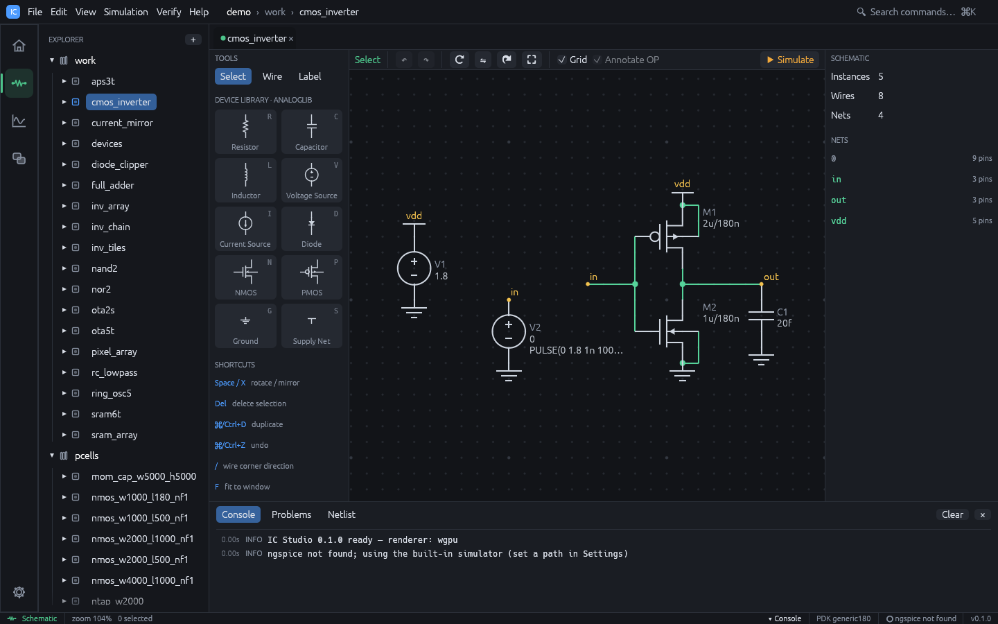
Schematic editor

  • Left panel: Tools (Select, Wire, Label), the Device Library with one tile per primitive and its shortcut letter, and a short shortcut reminder.
  • Toolbar: the current tool, undo / redo, rotate, mirror, duplicate, fit, the Grid and Annotate OP checkboxes, and Simulate (F5).
  • Right panel: the property inspector.

Schematic coordinates are integer grid points. Keys act on the canvas only while the mouse is over it and no text field has focus.

Devices

KeyDeviceName prefixPinsDefault parameters
RResistorRp, nr=1k
CCapacitorCp, nc=1p
LInductorLp, nl=1n
VVoltage SourceVp, ndc=1
ICurrent SourceIp, ndc=1m
DDiodeDa, kmodel=dmod
NNMOSMd, g, s, bmodel=nmos w=1u l=180n m=1
PPMOSMd, g, s, bmodel=pmos w=2u l=180n m=1
GGroundGNDgnd(net 0)
SSupply NetVDDnetnet=vdd

Placing a device

  1. Press the device key (for example N) or click its tile in the Device Library.
  2. A ghost follows the cursor. Press Space to rotate or X to mirror it before placing.
  3. Click to place. The device snaps to the grid, gets the next free name (M1, M2, …) and is selected. The tool stays active, so further clicks place more copies.
  4. Press Esc or right-click to return to Select.

Wires

  1. Press W (or choose Wire).
  2. Click the start point, usually a pin.
  3. Click the next point. Each click adds an L-shaped pair of segments, horizontal first; press / to bend vertical first.
  4. The wire ends automatically when a click lands on a pin, a wire end or the interior of another wire. Otherwise keep clicking, and end with double-click, right-click or Esc.

Connections are live: pins that are not connected are drawn as small squares, and a junction dot appears where three or more connections meet. Hovering or selecting a wire highlights its whole net.

Net labels and net names

  1. Press T (or choose Label). A Net: field appears in the left panel (default net1).
  2. Type the name and click on a pin or wire to attach the label. Labels connect only at their exact grid point.
  3. A trailing number is incremented after each placement (net1, net2, …), which is handy for buses of labels.

Labels with the same name are the same net, so labels connect parts of a schematic without wires. Net names are chosen in this order: the Ground symbol (net 0), the Supply Net symbol’s net parameter (blank means vdd), net labels, then automatic names (net1, net2, …).

Notes:

  • Only the Ground symbol makes net 0. A label called gnd is an ordinary net.
  • A Supply Net symbol only names a net. Place a voltage source on it to power it.
  • Two different names on one net produce the warning “Net names ‘a’ and ‘b’ are shorted together”.

Selecting and editing

ActionHow
Select one objectClick it (labels take priority over wires, wires over devices)
Add or remove from selectionShift+click or Ctrl+click
Box selectDrag on empty space (selects objects fully inside; Shift adds)
Select allCtrl+A
MoveDrag a selected object; attached wires stretch with moved pins
Rotate / mirrorSpace / X, or the toolbar buttons
DuplicateCtrl+D (copies offset by two grid points, renamed)
DeleteDel or Backspace
Undo / redoCtrl+Z / Ctrl+Shift+Z or Ctrl+Y
Fit to windowF
CancelEsc cancels a wire, then returns to Select, then clears the selection

Property inspector

Select a single device to edit it in the right panel. Values are SPICE strings typed as they would appear in a netlist, with SPICE scale suffixes: 10k, 2.2p, 180n, 1meg.

  • Name: the instance name. It must be unique; it also ties the device to its layout instance.
  • Device fields: Resistance, Capacitance, Inductance / L, Model, Width, Multiplier, Net name (supply).
  • Sources: DC value, AC magnitude (for AC analysis, e.g. 1) and Transient (e.g. PULSE(0 1 0 1n 1n 5n 10n); SIN(...) and PWL(...) also work).
  • Orientation and Position, and a Connections list showing the net on each pin.

With nothing selected, the inspector shows statistics (instances, wires, nets), the list of nets with their pin counts, and any Warnings (unconnected pins, duplicate names, shorted net names).

The Problems tab of the bottom panel runs the schematic checker on the active cell as you edit: missing ground, bad or duplicate names, missing or invalid values, shorted devices, voltage-source loops, floating nets, dangling wires and more. Click a finding to select its devices. Tools > Check Schematic runs the check on demand, and File > Check and Save saves only when there are no errors. See Check Schematic for every check.

Netlist

The Netlist tab of the bottom panel shows the SPICE deck of the active cell, updated as you edit. Export it with File > Export > SPICE netlist…. The netlister writes:

  • R1 p n value, C..., L...
  • V1 p n DC <dc> [AC <ac>] [<tran>], likewise for current sources
  • D1 a k dmod
  • M1 d g s b <model> w=... l=... [m=...]; an unconnected bulk pin is tied to the source
  • default level-1 models nmos, pmos and dmod when they are used. With a PDK model library, MOS models map to the PDK devices (subcircuit devices get an X prefix) and the library is loaded at the chosen corner.

Operating point annotation

After an operating point simulation, Annotate OP (on by default) shows each node voltage as a tag on the schematic and the current id=... under each transistor and diode.

OP annotation

Cross-probing

When a cell has both a schematic and a layout, selecting devices in one editor selects the devices with the same names in the other. Unit fingers of a matched device (M1.1, M1.2, …) map back to M1.

Simulation

The Simulation workspace (Ctrl+3) sets up and runs analyses of the active cell’s schematic and shows the results.
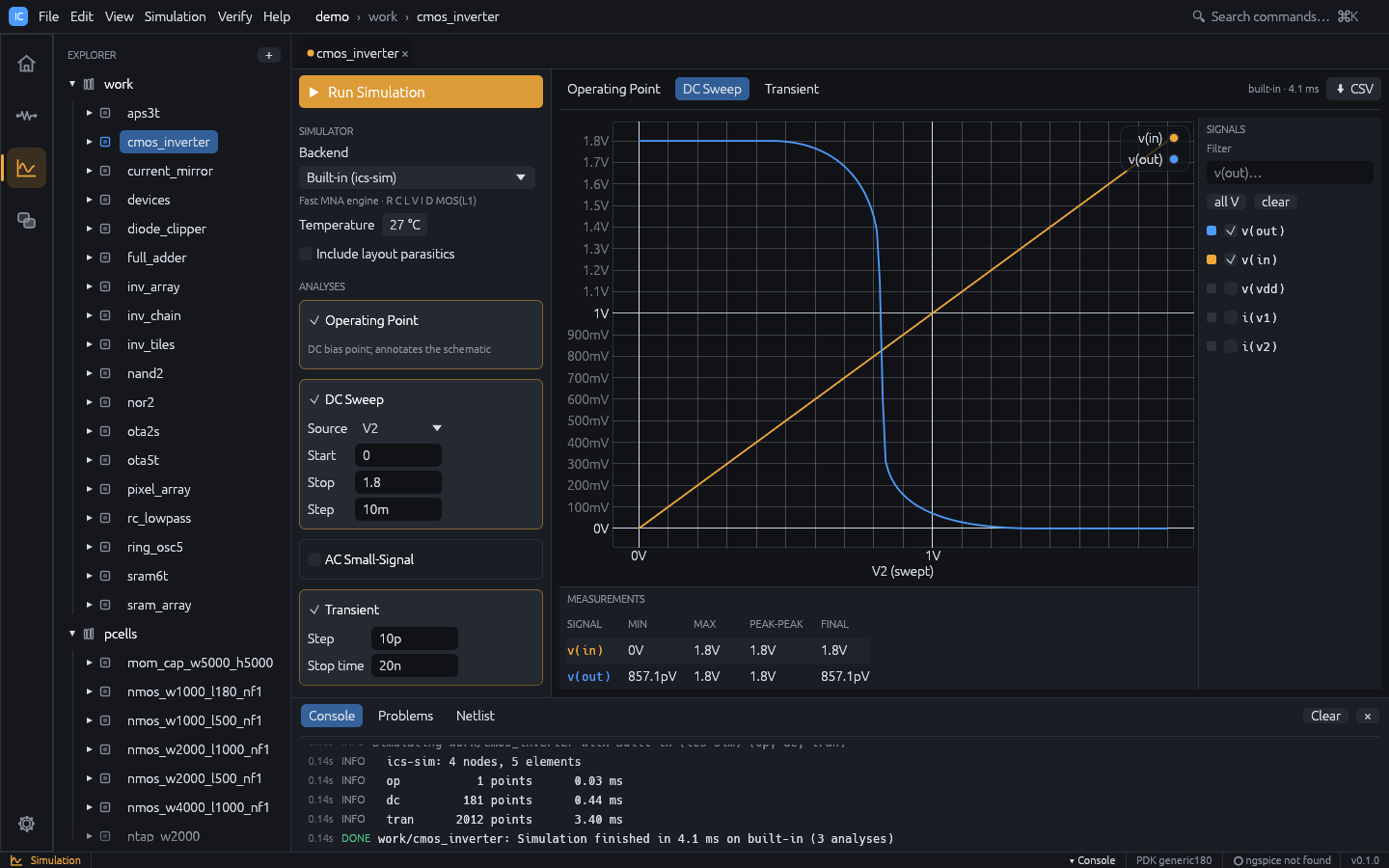
Simulation

Running a simulation

  1. Open a cell with a schematic and switch to the Simulation workspace.
  2. In Analyses, tick the analyses to run and fill in their fields.
  3. Press Run Simulation, F5 or Ctrl+Enter (also Simulation > Run or Simulate in the schematic toolbar).

Simulation runs in the background. Starting it from another workspace switches to the Simulation workspace. Errors appear in a red Simulation error box and in the console.

Setup panel

Simulator

FieldMeaning
BackendBuilt-in (ics-sim) (default) or ngspice
CornerModel corner of the PDK model library; shown only when the technology’s models have corners (default: the library’s default corner)
Temperature-55 to 200 °C, default 27 (written as .temp)
Include layout parasiticsAdd parasitics extracted from the cell’s layout (see below); disabled when the cell has no layout

The line under the backend shows whether ngspice was found, or that PDK models need ngspice when the technology has a model library. Set the ngspice path in Settings (see Installation).

Analyses

AnalysisFields (defaults)Notes
Operating Pointnone (on by default)Annotates the schematic
DC SweepSource, Start 0, Stop 1.8, Step 10mSource is any V or I source in the schematic
AC Small-SignalStart freq 1, Stop freq 10g, Points/dec 20Decade sweep; give a source an AC magnitude
TransientStep 10p, Stop time 20nGive a source a Transient waveform

Fields with an invalid value turn red; validation messages appear under the card.

Extra SPICE lines

Lines in this collapsible section are appended verbatim to the deck before the analyses, for example .options reltol=1e-4. Show netlist displays the generated deck next to the results.

The setup (backend, corner, analyses, temperature, parasitics flag, extra lines and the sweep setup) is saved per cell in sim.json.

Results

Each analysis has its own tab: Operating Point, DC Sweep, AC, Transient. The tab bar shows the backend and run time, and CSV exports the current dataset (AC values as name_re / name_im columns).

Waveforms

  • Signals (right): tick signals to plot. Filter narrows the list, all V selects every node voltage, clear clears the selection. By default v(out), v(in), v(vout) and v(vin) are shown when present, otherwise the first three voltages. The selection is kept per analysis between runs. Waveforms plotted from the Waveform Calculator appear here as signals named after their expression.
  • Compare runs (above the signal list): the earlier runs of the cell. Tick one to draw its signals dashed on the same plot and list them in the measurements (see Results Browser).
  • Plot: DC and transient results share one plot. AC results are a Bode pair: Magnitude (dB) over Phase (°) on a logarithmic frequency axis, with linked zoom and cursor. Hover a trace to read values. Scroll to zoom, drag to pan, double-click to reset.
  • Measurements (bottom), one row per plotted signal:
    • DC and transient: MIN, MAX, PEAK-PEAK, FINAL.
    • AC: GAIN @ fstart, PEAK, f -3 dB, UNITY GAIN f.
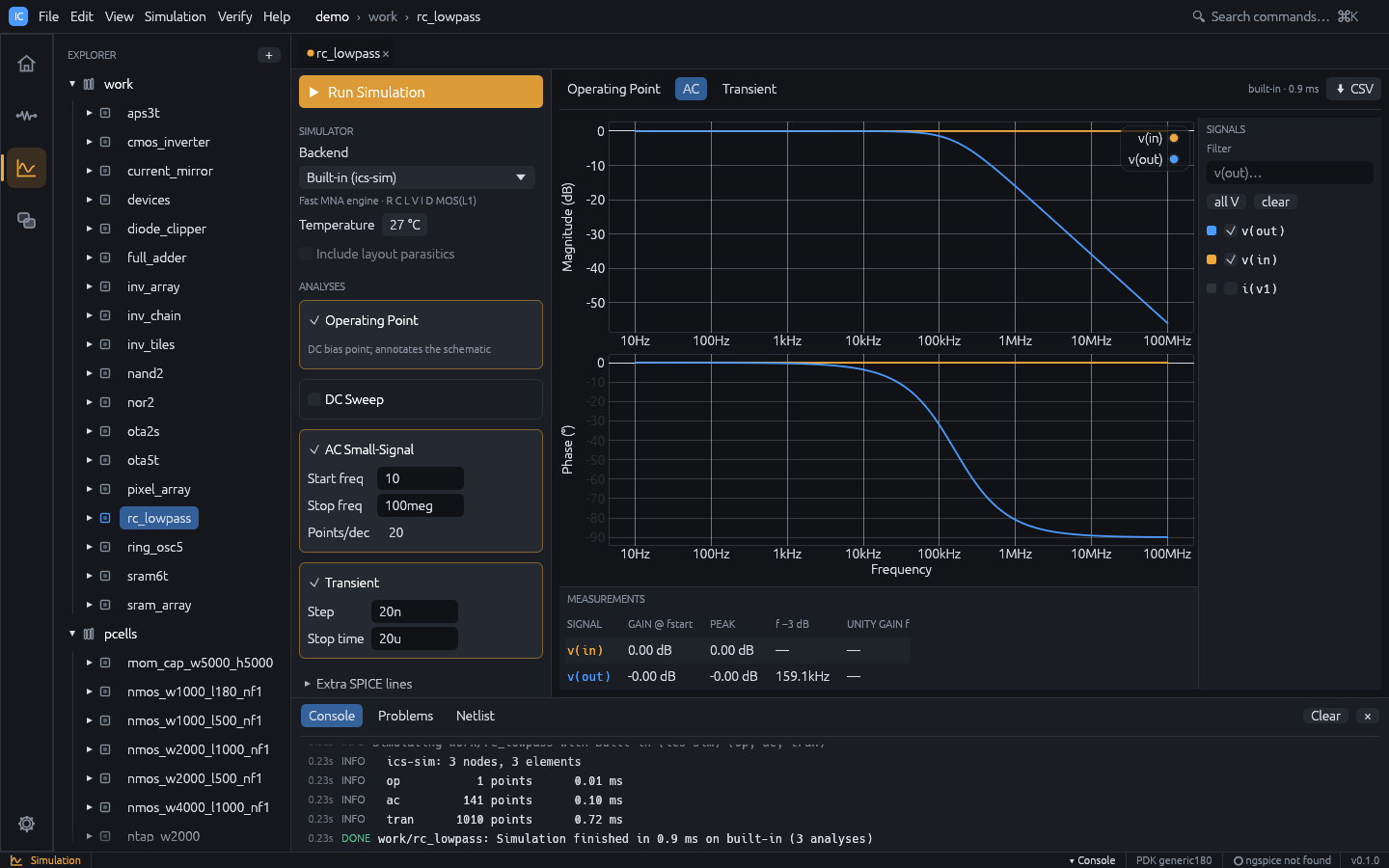
AC analysis of the RC low-pass

Operating point

The Operating Point tab lists node voltages and branch currents, and per device:

  • MOS: region (cutoff, saturation, triode), id, vgs, vds, vth, gm, gds
  • diode: vd, id, gd
  • resistor: v, i, p

Device details come from the built-in engine only. The node voltages are also drawn on the schematic (see Schematic).

Example: transient of the RC low-pass

  1. Run ic-studio --demo --cell rc_lowpass --workspace simulation.
  2. The cell has Operating Point, AC and Transient set up. Press F5.
  3. Open the AC tab: the f -3 dB column shows about 159 kHz for v(out).
  4. Open the Transient tab to see the input pulse and the filtered output.
  5. To change the input, go to the schematic (Ctrl+2), select the source, edit Transient, and press F5 again.

Measurements, corners and Monte Carlo

  • Tools > Waveform Calculator evaluates expressions on the results, such as bandwidth(v(out)/v(in)), risetime(v(out)) or phasemargin(v(out)), and plots derived waveforms. See Waveform Calculator.
  • Tools > Corner / Sweep Manager runs the setup over model corners, temperatures and parameter values, and Monte Carlo variations, in parallel; specs with limits are checked on every point, with statistics, yield, overlaid waveforms and an HTML datasheet. See Corner / Sweep Manager.
  • Tools > Results Browser keeps earlier runs for comparison, for example the schematic against the post-layout simulation.

Post-layout simulation

When Include layout parasitics is ticked and the cell has a layout, IC Studio extracts the layout, matches its nets to the schematic through LVS and adds to the deck:

  • wire capacitance to substrate (Cpar_*),
  • lateral and overlap coupling capacitance between nets (Cc_*),
  • MOS drain / source junction sizes (ad as pd ps) from the drawn diffusion,
  • an RC network of wire, via and gate resistance (Rpar_*), with each MOS terminal moved to the nearest node of its net.

Coupling to a layout net with no schematic counterpart is lumped to ground. The console shows a one-line summary. For a useful result, the layout should be LVS clean (see Verification). From the command line: ics sim <project> <cell> --parasitics.

Backends

Built-in engine

A modified nodal analysis engine written in Rust. It supports:

  • elements R C L V I D M (no subcircuits or behavioural sources),
  • sources: DC, AC mag [phase], PULSE(v1 v2 td tr tf pw per), SIN(vo va freq td theta), PWL(t v ...),
  • directives .model, .op, .dc, .ac, .tran, .temp, .end; other dot lines such as .options, .param and .subckt are ignored, and a deck with .include or .lib is rejected (model libraries need ngspice),
  • diode model (is, n, cjo) and MOS level 1 (vto, kp, lambda, gamma, phi, tox, cgso, cgdo, cj, cjsw) with instance parameters w l m ad as pd ps.

The generic nmos / pmos models the netlister writes use vto = ±0.45 and kp = 280u / 70u; a MOS model parameter left out defaults to vto = ±0.7, kp = 2e-5.

ngspice

With the ngspice backend, IC Studio runs ngspice in batch mode and reads its raw output. ngspice reads the deck itself, so subcircuit devices (X), .include and .lib model libraries of a PDK work; IC Studio only takes the analyses (.op, .dc, .ac, .tran) from the deck when the setup lists none.

Layout editor

Open a cell’s layout view (or press Ctrl+4 with a cell open). Layout coordinates are database units (1 dbu = 1 nm in the generic technology, y pointing up); the inspector shows µm. Every point snaps to the snap grid (the Snap field in the toolbar, a multiple of the technology grid). The editor follows Virtuoso conventions: two-click commands with a prompt in the top-left corner of the canvas, bindkeys (S stretch, M move, C copy, Shift+C chop, O via, T layer tap, u undo, Z zoom box, W previous view, q properties, F3 command options, F4 partial select, …; see Keyboard shortcuts), floating option forms, a middle-click pop-up menu, gravity snapping and design-rule-driven feedback. In the Layout workspace the menu bar adds Create and Options menus, and Edit, View and Verify gain the layout commands; every item shows its bindkey, and the command palette lists them as “Layout

: ”.

Layout editor

  • Left panel: Hierarchy (drawn levels and the tree of placed cells), Layers, and the options of the current tool.
  • Toolbar: undo / redo, the tools (Select, Stretch, Move, Copy, Rectangle, Polygon, Path, Label, Via, Instance, Chop, Ruler), fit, Zoom box, Prev view, Grid, Snap, Gravity, DRD, Constraints, Magnet, Live DRC, Flylines, and GDS to export the cell.
  • Status bar: X / Y of the cursor; while a command is in progress dX, dY and Dist from its reference point; Sel: n (Sel(P): n for a partial selection); Cmd: the current tool; and a mouse L: … M: … R: … line telling what each button does now.
  • Right panel: cell statistics or the inspector, Edit operations, Layer operations, and the verification sections (see Verification).

Layers

  • Click a layer row to make it the active layer; new shapes are drawn on it.
  • Click the eye to show or hide a layer. Click the small box left of the eye to make a layer selectable or not: shapes on non-selectable (or hidden) layers are drawn but cannot be picked, like Virtuoso’s LSW. AV / NV show / hide every layer, AS / NS make every layer selectable / not.
  • Filter narrows the list by name; Instances selectable controls whether placed cells can be picked.
  • Each row shows the fill pattern, the name and the GDS layer/datatype. Hover a row to see its minimum width and spacing.

Drawing

Keys act on the canvas only while the mouse is over it.

ToolKeyHow to use
SelectEscClick, Shift/Ctrl+click, or drag a box
StretchSClick an edge or vertex of a shape, then the destination (or drag it). Or drag a box away from any edge: the vertices inside become the partial selection; then click a reference point and the destination
RectangleRDrag from corner to corner, or click two corners; the size is shown
PolygonShift+PClick each vertex; Enter, double-click or right-click closes it
PathPClick points; Enter, double-click or right-click finishes it
LabelLType the Text in the left panel, click to place
ViaOPick a via in the left panel; click for one cut, drag to fill an area
InstanceIPick a cell or PCell in the left panel, click to place
ChopShift+CDrag or click a box; it is cut out of the selected shapes (or of every selectable shape it touches)
RulerKDrag or click two points; rulers stay until Shift+K

While drawing a polygon or path, Backspace removes the last point and Esc cancels.

  • Gravity (on by default, G toggles) snaps the cursor to vertices (diamond marker) and edges (circle marker) of nearby shapes and instance boxes, so new geometry abuts exactly.

  • DRD (design-rule-driven editing, on by default) shows the minimum-spacing halo of a rectangle being drawn and marks in red every gap to a same-layer shape that is closer than the minimum spacing, and shapes narrower than the minimum width. It works while drawing rectangles and paths, moving, copying and pasting. Neighbours inside placed cells count too (at any depth), as do the shapes around a cell edited in place; a moved or pasted instance is checked by the shapes along its outline.

  • Magnet (on by default) pulls a shape being drawn or moved to exactly the minimum spacing from its neighbours when it comes close.

  • Live DRC (on by default) checks the rule deck around every edit; see Live DRC.

  • Layer tap: T makes the layer of the shape under the cursor the active layer.

  • Changing metal while routing: with the Path tool, press + (or = / PageUp) to end the path at the cursor, drop the via to the routing layer above and continue on it; - (or PageDown) goes down.

  • Polygons are Manhattan by default: each point is aligned horizontally or vertically to the previous one. Hold Shift (or Ctrl) while clicking for any angle. The closing edge gets an extra corner so a Manhattan outline stays Manhattan.

  • Paths are always Manhattan. Width (nm) in the left panel sets the width; 0 uses the layer’s minimum width. Path ends are extended by half the width.

  • Labels on a routing layer name the net under them (used by extraction and LVS).

  • Vias come from the technology (bottom layer, cut, top layer); dragging an area fills it with as many cuts as fit.

Rectangle step by step

  1. Click the metal1 row in Layers.
  2. Press R and drag on the canvas.
  3. Press Esc to return to Select, click the rectangle and type exact coordinates in the inspector (x0, y0, x1, y1 in µm).

Selecting and editing

ActionHow
SelectClick; the smallest shape under the cursor wins. Click the same spot again to cycle through the items under it
Add / removeShift+click or Ctrl+click
Box selectDrag on empty space: left to right selects items fully inside, right to left (dashed box) every item it touches; Shift adds
Select allCtrl+A
MoveDrag a selected item; or M, click a reference point, click the destination; or nudge with Shift+arrow keys (10 snap steps). Right-click while moving rotates 90°, Shift+right-click flips sideways
CopyC, click a reference point, then click destinations (each click places another copy, Esc ends); rotate / flip as for Move
StretchS, click an edge or vertex, click the destination; with a partial selection, click a reference point, then the destination; or drag a box over several edges (see below)
Yank / pastey or Ctrl+C copies the selection (Ctrl+X cuts it); Shift+Y or Ctrl+V attaches it to the cursor, click to place. The clipboard also works between cells
Merge / chopShift+M / Shift+C
ReshapeWith one shape selected, drag a vertex handle (square) or an edge handle (round); Manhattan shapes stay Manhattan
Rotate 90° / flipShift+O, or Rotate 90°, Flip X, Flip Y
Deselect allCtrl+D
DeleteDel or Backspace
Undo / redou / Shift+U, or Ctrl+Z / Ctrl+Shift+Z or Ctrl+Y
DescendShift+X over an instance (or with one selected) opens its cell on its own; Shift+B returns. Shift+T shows the hierarchy tree
FlipCtrl+J flips the selection sideways, or what is being moved or copied
Edit in placex over an instance (or with one selected) edits its cell, or the array element under the cursor, inside the parent: the surroundings stay visible, dimmed, in the parent’s orientation, and DRD checks against them. Shift+B or Return in the toolbar goes back
Open a placed cellDouble-click the instance, or Open in the inspector
Pop-up menuMiddle-click, or right-click when no command point is pending: Move, Copy, Stretch, Delete, Properties, Rotate 90°, Merge, Yank, Paste, Descend Edit, Return, Fit All, Previous View, plus Edit In Place. With nothing selected, the item under the cursor is selected first

Partial selection

F4 (or Edit > Toggle Partial Select) toggles partial selection. In Select, a click near an edge selects that edge (both its vertices) or a vertex; Shift+click adds or removes; a drag box selects the vertices inside it (items entirely inside are taken whole). Selected edges and vertices are highlighted and the status bar shows Sel(P): n.

Press S, click a reference point, then the destination: every selected vertex moves, and Manhattan shapes stay Manhattan (adjacent edges slide along). Dragging a partially selected shape in Select stretches it too. Esc clears the partial selection.

Forms

Each key opens a floating form and closes it again:

KeyForm
qEdit Object Properties: the inspector for the selection
F3Options of the current command (path width, label text, via, instance placement; snap and gravity for commands without options)
eDisplay Options: grid, display levels From 0 To N, flylines, clear rulers
Shift+ELayout Editor Options: snap spacing, gravity, DRD, instances selectable, partial selection, default path width

The Edit section of the right panel (shown when something is selected) also has:

  • Flatten: replace the selected instances with their contents (one level).
  • Make cell: move the selection into a new cell and place an instance of it.
  • Merge: union the selected shapes per layer.
  • Size with Apply: grow (positive µm) or shrink (negative) the selected shapes.
  • Align (two or more items): align left, centre or right edges, bottom, centre or top edges; Space X / Space Y spread three or more items with equal gaps.
ActionHow
ZoomCtrl+wheel or pinch, [ in / ] out at the cursor, Shift+Z out (Conventional profile: the wheel)
Zoom boxRight drag, or Z (or Zoom box), then drag or click two corners
Previous / next viewW / Shift+W (or Prev view)
FitF
PanWheel (up / down), Shift+wheel (sideways), middle drag, or the arrow keys
Pop-up menuMiddle-click (or right-click when no command point is pending)

These are the Virtuoso interaction profile, the default. With Conventional (Settings > Interaction) the wheel zooms and a right drag pans.

Bindkeys go to the canvas while the mouse is over it, and stay with it while one of its forms (q, F3, e, Shift+E) is open on top, until you click elsewhere in the window. A text field being typed in, or a focused control in a form under the mouse, gets the keys first.

Layer operations

With nothing selected, Layer operations computes Boolean results:

  1. Choose layer A, an Operation (AND, OR, NOT, XOR, SIZE) and layer B (or a distance By in µm for SIZE).
  2. Choose the Output layer.
  3. Keep Include hierarchy (flattened) checked to include placed cells.
  4. Press Run. The result shapes are added to the output layer and selected.

Boolean operations, Merge, Size and Chop handle any-angle geometry (45° and arbitrary edges, from GDS / OASIS or the polygon tool) exactly. Crossings that fall between grid points snap to the nearest database unit. When sizing, horizontal, vertical and 45° edges move by the given distance and corners of 90° or more stay sharp. Results with holes are cut into hole-free polygons.

Constraints, compaction and compare

These commands have no menu or bindkey; run them from the command palette, where they are listed as “Layout Assist: ”.

  • Symmetric About Vertical / Horizontal Axis, Keep Left / Bottom Edges Aligned, Keep Centres Aligned Vertically / Horizontally and Fix In Place add a constraint to the selected items. Moving one member moves the others so the constraint keeps holding. Infer Constraints From Schematic adds symmetry constraints for the schematic’s matched devices; Remove Constraints clears them. The Constraints checkbox in the toolbar draws them, and the Constraints section of the right panel lists them, with Snap for one that no longer holds.
  • Compact (Left, Then Down) and Compact Left / Right / Down / Up slide the cell’s top-level items toward one side as far as the spacing rules allow. Connected geometry and the members of a constraint move together.
  • Compare With Saved and Compare With Git HEAD draw the geometry added and removed since the last save or the last commit; Next Difference steps through them.

Hierarchy

Hierarchy

Placing a cell or an array

  1. Press I. The left panel lists PCell variants and Place cell (every other cell with a layout that would not create a cycle).
  2. Pick a cell, set Rotation, Mirror about x, Columns and Rows. Array elements abut at the cell’s extent.
  3. Click to place.

Select an instance to edit its position, rotation and mirroring in the inspector. Check Array to turn it into an array (GDS AREF) with Columns, Rows, Column pitch and Row pitch.

Drawn depth

The levels field in Hierarchy (keys 0 to 8, and 9 for all levels) sets how many levels of placed cells are drawn with their contents (Shift+F all levels, Ctrl+F top level only). Deeper instances are drawn as labelled boxes. Missing cells are drawn in red.

Large designs stay fast: cells that are small on screen collapse to boxes and tiny shapes to dots.

8192 inverters

The hierarchy tree (Edit > Hierarchy Tree, Shift+T) lists the cells placed in the current cell with their counts; click one to open it. Tools > Hierarchy Browser shows the whole project’s layout hierarchy with where-used lists (see Tools).

Generators and fill

The Tools menu also adds geometry to the active layout, each as one undoable step:

  • Layout Generators > Guard Ring: a p+ substrate or n+ nwell ring with contacts and a metal1 strap around an area or the selection;
  • Layout Generators > Via Array: via arrays on every overlap of two layers, or filling an area;
  • Layout Generators > Matched Placement: common-centroid, interdigitated or 2-D common-centroid placement of matched transistors with dummies;
  • Layout Generators > By Example: place the devices like a finished cell with the same circuit (matched by topology), copying its wells, implants and taps, and optionally route;
  • Dummy Fill: fill squares to meet a density rule.

See Tools for the options.

PCells

PCells

Parametric cells are generated from the technology and stored as ordinary cells in the pcells library (for example nmos_w1000_l180_nf2).

PCellParametersDefaults
nmosW, L, fingers, deviceW 1 µm, L 0.18 µm, 1 finger
pmosW, L, fingers, deviceW 2 µm, L 0.18 µm, 1 finger
poly_resW, LW 0.4 µm, L 5 µm
mom_capW, H5 µm x 5 µm

Device appears when the technology is a PDK with several MOS devices of that polarity (for example low- and high-Vt variants): the PCell then draws that device’s marker layers, and the variant name ends with the device name. The default is the PDK’s first device.

To place one, press I, choose the PCell in the left panel, set its parameters and click. To change a placed PCell, select it, edit the parameters in the PCell section of the inspector and press Apply. Well and substrate taps (ntap, ptap) are created by schematic-driven layout; their parameters can be edited in the inspector the same way.

SKILL scripts

Tools > Load SKILL (.il) runs a Cadence SKILL file on the project; ics skill and the MCP tool run_skill do the same from the command line and from agents. Printed output goes to the log, every changed layout can be undone, and geGetEditCellView() returns the cell open in the editor.

The CIW tab of the bottom panel (Tools > SKILL CIW, or “CIW” in the command palette) is an interactive SKILL prompt like Virtuoso’s Command Interpreter Window. Variables, procedures and open cellviews persist between commands and include everything defined by files loaded with Tools > Load SKILL; opening another project starts a fresh session. Enter runs the line, a line with unclosed parentheses or strings continues on the next one (the prompt shows ...), and Up / Down recall earlier commands.

cv = dbOpenCellViewByType("work" "pad" "layout" "maskLayout" "w")
for(i 0 3
  dbCreateRect(cv list("metal1" "drawing") list(i*2:0 i*2+1:1)))
dbCreateInstByMasterName(cv "work" "via_cell" "layout" "I0" 0:5 "R90")
printf("%d shapes\n" length(cv~>shapes))

Supported:

  • syntax: C style f(a b) and Lisp (f a b) calls, infix operators, x:y points, obj~>prop, tbl[key], 'quote, ?key arguments, ; and /* */ comments, scale factors such as 1.5u;
  • control: if / then / else, when, unless, cond, case, while, for, foreach (also mapcar and tables), let, prog / return, setof, exists, errset, error;
  • procedure / defun with @optional, @key, @rest, lambda, funcall, apply, mapcar, load; list, string, math and printf / sprintf built-ins, makeTable tables and disembodied property lists;
  • layout: dbOpenCellViewByType ("r", "w" clears the layout, "a" appends; libraries and cells are created on demand), dbCreateRect, dbCreatePolygon, dbCreatePath, dbCreateLabel, dbCreateInst, dbCreateInstByMasterName, dbCreateSimpleMosaic, dbDeleteObject, dbMoveFig, dbCopyFig, dbFindAnyInstByName, dbGetOverlaps, dbTransformPoint / dbTransformBBox; layer Boolean operations dbLayerAnd, dbLayerOr, dbLayerXor, dbLayerAndNot (cv layer shapes1 shapes2) and dbLayerSize (cv layer shapes size), which add the result to layer and return the new shapes (any-angle geometry included); dbSave and dbClose do nothing (save the project). Shape, instance and cellview properties (bBox, points, layerName, xy, orient, shapes, instances, …) can be read, and the geometric ones set.

Coordinates are in µm. A layer is a name, list(name purpose) or a layer index; a purpose other than drawing first looks for a layer named name.purpose or name_purpose. Variables are dynamically scoped as in .il files. Not supported: schematic views, PCell definitions (pcDefinePCell), interactive hi* / le* forms and SKILL++ (.ils) lexical scoping.

GDSII

  • File > Import > GDSII / OASIS… reads a GDS or OASIS file into a new library with full hierarchy.
  • GDS in the toolbar or File > Export > Cell GDSII… writes the cell and every cell it places; Export > Library GDSII… writes every layout in the project. Cell OASIS… and Library OASIS… write OASIS instead.

Layers are mapped by GDS layer / datatype. Layers the technology does not have are added to it on import, so nothing is lost. A stream layer map (Tools > Stream Layer Map, or a Virtuoso layer map file) renumbers layers on export, maps other numbers onto technology layers on import, or drops them.

Verification: DRC, extraction and LVS

The verification tools are in the Verify menu and in the right panel of the Layout workspace. They run in the background on the flattened layout of the active cell; while one runs, the panel shows its progress and a Cancel button. After you edit the layout, the panel notes that results are out of date.

Design rule check (DRC)

DRC

  1. Open the cell’s layout.
  2. Press Run DRC in the Design Rule Check section (or Verify > Run DRC).
  3. The result is either No violations or a list grouped by rule, with a count per rule. Markers are drawn on the canvas.
  4. Expand a rule to see its description and the violation locations; click one to zoom to it.
  5. Clear removes the results and markers.

The rules come from the technology’s deck. Expand Rule deck to view and edit it in place: Run DRC uses the edited text right away, Save to technology stores it in the project’s tech.json, and Reset replaces it with the deck derived from the technology’s layer and via rules. Syntax errors are listed by line. See Technology for the deck syntax. Rule Designer… (also Tools > DRC Rule Designer) edits the deck as forms and self-tests every rule on generated patterns; see DRC Rule Designer.

A layer that fails a density rule can be filled with Tools > Dummy Fill (see Dummy Fill).

DRC checks Manhattan geometry; other shapes are skipped and counted. Distances between corners are Euclidean.

Live DRC

The Live DRC checkbox in the layout toolbar re-checks the deck around every edit in the background and draws the violations as dashed boxes as they appear; hover one to see its rule. Quick Fix (Ctrl+.) on a violation offers candidate edits of top-level shapes (reshape, move or add), each checked with DRC first and marked clean or with the number of new violations it causes; it turns live DRC on when it is off. Fix All Violations (command palette) applies fixes until none helps any more, as one undoable step. Geometry inside placed cells is not changed.

Connectivity extraction

  1. Press Extract in the Connectivity section (or Verify > Extract Nets).
  2. The summary shows the number of nets and NMOS / PMOS transistors.
  3. Click a net in Nets to highlight it. Check Pick nets and click a shape on the canvas to highlight the net it belongs to.
  4. Devices lists each transistor with W, L and its terminal nets; click one to zoom to its gate.

Tools > Net Browser lists the extracted nets in a sortable table with their layers, area, transistor terminals and wire capacitance; click one to highlight it and zoom to it (see Net Browser).

How the extractor works:

  • Conducting layers are the layers joined by vias. Diffusion is active minus poly.
  • A transistor is poly over active. It is PMOS when it is inside pplus (or inside nwell when there is no implant). L is measured across the gate; W is area / L.
  • Net names come from labels in the top cell on conducting layers. Unnamed nets are called netN.
  • Warnings report labels not on conducting geometry, two labels shorted together, and a label on several unconnected pieces.

Layout versus schematic (LVS)

LVS

  1. The cell needs both a schematic and a layout. Device names do not have to match, but labels on the layout’s pins (in, out, vdd, …) help: equal net names anchor the comparison.

  2. Press Run LVS (or Verify > Run LVS).

  3. The result is Layout matches schematic or a list of differences, each tagged:

    • [missing]: a schematic device not found in the layout,
    • [extra]: a layout device not in the schematic,
    • [param]: W or L differ by more than 1 %,
    • [net]: a net whose connections differ.

    Click a difference with a location to zoom to it.

Comparison rules:

  • Only MOS transistors are compared. Voltage and current sources are ignored; other schematic devices (R, C, diodes) are reported as not extracted.
  • Parallel devices with the same terminals and L are merged and their widths summed, so multi-finger layouts match single schematic devices; the schematic m multiplies W.
  • Bulk terminals are ignored.
  • Devices that are always off (gate tied to bulk), such as dummy fingers, are dropped.
  • Net names are compared case-insensitively; 0, gnd and vss are treated as the same.

The demo cell cmos_inverter deliberately has LVS findings (a PMOS width and the load capacitor); nand2, nor2, ring_osc5, current_mirror, ota5t, sram6t, aps3t, full_adder and ota2s are clean.

Sign-off with external tools

The built-in checks are fast and good for iterating. For sign-off, a technology can list runsets that run a foundry or PDK deck in an external tool:

ToolChecksDeck
KLayoutDRC, LVSKLayout .drc / .lvs script
Siemens CalibreDRC, LVSSVRF rule file
netgenLVSnetgen setup file (compares IC Studio’s extraction with the schematic)
built-inDRCIC Studio or SVRF deck file, run on the built-in engine

In the Layout workspace, the Sign-off section appears when the technology has runsets. Pick a Runset and press Run (or Verify > Run Sign-off Runset). IC Studio writes the cell and every cell it places to <cell>.gds in a new temporary folder, plus the schematic as a .subckt for LVS, runs the tool there and reads its report:

  • DRC violations appear as markers on the canvas, like the built-in DRC. Violations the tool reports inside sub-cells keep sub-cell coordinates and name the cell.
  • LVS shows whether the layout matches and the tool’s messages.
  • The folder (shown under the result) keeps the inputs, reports and the tool’s log.

How each tool is called:

  • KLayout: klayout -b -r DECK -rd input=CELL.gds -rd topcell=CELL -rd report=FILE, plus -rd schematic=CELL_sch.cir for LVS and the runset’s vars. The variable names can be changed with klayout = { input = "...", topcell = "...", report = "...", schematic = "..." }.
  • Calibre: a control file sets LAYOUT PATH, LAYOUT PRIMARY, LAYOUT SYSTEM, the ASCII results database (DRC) or SOURCE PATH / LVS REPORT (LVS), adds #DEFINE for each var and INCLUDEs the deck. The deck itself must not set these statements. Then calibre -drc -hier or calibre -lvs -hier -spice.
  • netgen: netgen -batch lvs "CELL_lay.cir CELL" "CELL_sch.cir CELL" SETUP REPORT.

The schematic netlist leaves out the element letters in the runset’s skip (default V and I) and names the ground net ground (default gnd). Executables are found on the usual install paths and PATH; set ICS_KLAYOUT, ICS_CALIBRE or ICS_NETGEN to override them.

Runsets come from a PDK file ([[signoff]]) or the signoff array in tech.json:

"signoff": [
  {"name": "KLayout DRC", "tool": "klayout", "check": "drc", "deck": "/pdk/rules.drc",
   "vars": {"feol": "true"}},
  {"name": "Calibre LVS", "tool": "calibre", "check": "lvs", "deck": "/pdk/calibre.lvs",
   "skip": ["V", "I", "C"]}
]

From the command line

ics drc myproj nand2 [--deck rules.drc]   # exit code 1 on violations
ics extract myproj nand2                  # extracted SPICE netlist
ics lvs myproj nand2                      # exit code 1 on differences
ics signoff myproj nand2                  # list the sign-off runsets
ics signoff myproj nand2 "KLayout DRC"    # run one; exit code 1 on violations / mismatch

These exit codes make the checks usable in CI. See Command line.

Schematic-driven layout

IC Studio can build a layout from a schematic: it places the transistors as PCells, shows the connections still to be made as flylines, and routes them.

Schematic-driven layout

Step by step

  1. Draw and simulate the schematic. Give the external nets labels (in, out, …); use the Ground and Supply symbols for the rails.
  2. With the cell active, choose Verify > Generate Layout from Schematic. The cell gets a layout view if it has none, and the Layout workspace opens with flylines on.
  3. Inspect the placement. Move devices if you want; their names keep the link to the schematic.
  4. Choose Verify > Route Flylines to route the remaining connections.
  5. Add pin labels on metal for the external nets (Label tool, L) so that LVS can anchor them.
  6. Run DRC and LVS (see Verification), then simulate with Include layout parasitics.

Each step can be undone with Ctrl+Z. The console lists what was placed, skipped, matched and routed.

Demo: auto P&R

The demo cells full_adder (28 transistors) and ota2s (two-stage OTA with a common-centroid input pair and mirror) have layouts made only by this flow. Clear one (Ctrl+A, Delete) and run the two commands above to watch it happen. The demo gallery has a complete script.

Placement

  • Each NMOS and PMOS becomes a PCell instance named after the schematic device (M1). W and L come from the device’s w and l parameters; m multiplies the device. Devices wider than 5 µm are split into fingers. With a PDK, the schematic model selects the PCell’s device (and its marker layers, such as lvtn for a low-Vt model).
  • PMOS devices form a row above the NMOS row, gates facing the channel between the rows.
  • Neighbouring devices of the same type and width that share a source / drain net are abutted with shared diffusion.
  • Wells and implants are merged across each row, and each row ends with a bulk tap (ntap in the PMOS row, ptap in the NMOS row) on the row’s bulk net.
  • Devices already in the layout (by name) are left alone, so you can generate again after adding devices to the schematic.
  • Devices without a layout generator (R, C, L, diodes, sources) are skipped and listed in the console.

Matched devices

Differential pairs and current mirrors are detected automatically:

  • Differential pair: two devices of the same type, W, L and m with a common source net that is not a rail, and different gates and drains.
  • Current mirror: devices of the same type and L with a common gate and source, where the gate is tied to one device’s drain.

You can also group devices explicitly by giving them the same match parameter, or opt a device out with match=none. The inspector shows only the standard parameters, so add match (and match_rows) to the device’s params in the cell’s schematic.json:

"params": { "model": "nmos", "w": "4u", "l": "500n", "m": "1", "match": "pair1" }

A matched group is split into equal unit fingers named <device>.<k> (for example M1.1, M1.2), placed in common-centroid order (ABBA). Groups of 8 units or more, or groups with match_rows=2, use two cross-coupled rows (ABBA / BAAB); match_rows=1 forces a single row. Each unit row is closed by dummy fingers at both ends whose gates are tied to bulk; LVS ignores them because they are always off.

The console reports each group, for example A, B: matched as ABBA (A = M1, B = M2), or why it could not be matched.

Flylines

The Flylines checkbox in the layout toolbar draws a dashed line, labelled with the net name, for every schematic connection that is not yet made in the layout. They update after every edit, so you can route by hand and watch them disappear.

Router

Route Flylines runs a maze router (A* search) over the routing metal layers above poly (metal1, metal2 and metal3 in the generic technology):

  • The routing grid is aligned to the device terminals; wires have one width that fits a via, with DRC spacing between tracks.
  • Existing geometry is avoided. Short nets are routed first; nets that block each other are ripped up and rerouted.
  • Metal1 is expensive and each higher layer has a preferred direction, so long runs move to upper metals.

Every named schematic net (labels and supplies; the ground symbol becomes gnd) that is fully connected after routing gets a text label at one of its terminals, unless the top cell already has a label of that name. The label goes on the first metal, or on the layer the PDK names for its net labels ([[pin_label]], e.g. Metal1.text in SG13G2), so external LVS decks see the layout’s ports with their schematic names.

The console summary gives the routed nets, connections, vias and rip-ups. Nets that could not be routed stay as flylines with a reason (terminals not on conducting geometry, or pieces not reached). Finish them by hand and route again.

Cross-probing

Select a device in the schematic and switch to the layout: the instances with the same name (including its unit fingers) are selected, and the other way round.

From the command line or an agent

ics route myproj nand2 --place   # place missing devices, route, save; exit 1 if nets remain

The MCP server offers generate_layout, flylines and route (see MCP server).

Technology

The technology (PDK) of a project lives in tech.json in the project folder. It defines the layers, their GDS numbers and display style, simple width / spacing rules, vias, electrical coefficients for parasitic extraction, and the DRC rule deck. A project without tech.json uses the built-in generic180 technology.

generic180

A generic 180 nm-class technology, used by new projects and the demo. 1 dbu = 1 nm, grid 10 nm.

LayerGDSLayerGDS
nwell1via18
active2metal29
nplus3via210
pplus4metal311
poly5boundary62
contact6text63
metal17

Routing layers are poly and metal1 to metal3. Vias: contact (active to metal1), polycon (poly to metal1), via1, via2.

tech.json

Top level:

FieldMeaning
nameTechnology name
dbu_per_umDatabase units per µm (1000 means 1 dbu = 1 nm)
gridSnap grid in dbu
layersArray of layers
viasArray of via definitions
drc_deckDRC deck text (optional; derived from the layer rules when absent)
capsPer-layer parasitic coefficients (optional)
rolesWhich layers and vias are the diffusion, poly, well, implants and contacts (optional; generic180 names by default)
rulesDevice rules used by the PCells, in dbu (optional)
devicesPDK MOS devices (optional; generic nmos / pmos when absent)
modelsPDK SPICE model library (optional; built-in level-1 models when absent)
signoffExternal DRC / LVS runsets (optional; see Verification)
pcell_layers, pin_labels, drc_extraExtra PCell layers, net label layers and deck lines, as [[pcell_layer]], [[pin_label]] and drc_extra of a PDK file (optional)
stream_mapGDSII / OASIS layer map for import and export: rows of layer, stream_layer, datatype (optional; see Stream Layer Map)

Layer:

{
  "name": "metal1", "gds_layer": 7, "gds_datatype": 0,
  "color": [80, 140, 255, 160], "fill": "hatch",
  "min_width": 230, "min_spacing": 230, "routing": true
}
  • fill: solid, hatch, backhatch, cross, dots or outline.
  • min_width, min_spacing: in dbu; 0 means not checked. min_area (optional): in dbu²; PCell contact plates and router via pads grow to reach it.
  • routing: a routing layer carries net labels and is used by extraction and the router.

Via: name, bottom, cut, top (layer names), cut_size, cut_spacing, enc_bottom, enc_top (dbu) and resistance (Ω per cut).

Parasitic coefficients (caps), one entry per layer: layer, area (aF/µm²), fringe (aF/µm of edge), coupling (aF; adds coupling * length / spacing for a parallel neighbour) and resistance (Ω per square).

DRC rule deck

The deck is plain text, one statement per line. # starts a comment. Lengths are in µm, areas in µm². Keywords and layer names are not case sensitive. Every rule can have an optional NAME: prefix; otherwise a name such as metal1.W or contact.EN.metal1 is generated. A #@ text line gives the next rule its description, reported with its violations instead of the generated one.

Rules

StatementChecks
width LAYER MINMinimum width
space LAYER MINMinimum spacing between shapes of one layer
separation A B MINMinimum spacing between A and B (B pieces that do not overlap A)
enclosure INNER OUTER MINOUTER must enclose INNER by MIN (INNER pieces that overlap OUTER)
extension A B MINA must extend past B by MIN (e.g. poly endcap over active)
area LAYER MINMinimum area
antenna METAL RATIOMaximum ratio of metal area to connected gate area (needs poly and active layers)
density LAYER MIN MAX WINDOW [STEP]Density between MIN and MAX percent (plain numbers, 0 to 100) in a sliding WINDOW x WINDOW µm window (STEP defaults to WINDOW/2)
flag LAYEREvery piece of LAYER is a violation (use it with a derived layer)

Derived layers

NAME = A and B
NAME = A or B
NAME = A not B        # A minus B
NAME = A xor B
NAME = A size DIST    # grow (negative DIST shrinks)
NAME = A wide MIN     # the parts of A at least MIN wide
NAME = A interact B   # pieces of A that overlap or touch B
NAME = A inside B     # pieces of A entirely inside B
NAME = A outside B    # pieces of A that do not overlap B
NAME = A enclose B    # pieces of A that contain a whole piece of B
NAME = A touch B      # pieces of A that touch B without overlapping it
NAME = A not interact B   # (also not inside, not outside, not enclose, not touch)
NAME = A area MIN MAX # pieces with MIN <= area < MAX (µm²; MAX may be inf)
NAME = holes A        # the enclosed empty areas of each piece of A
NAME = extents A      # the bounding box of each piece of A

A piece is an edge-connected part of a layer. Derived layers can use technology layers and derived layers defined earlier, and can be used in any rule. With flag, any derived layer becomes a check, for example floating poly:

floating = poly not interact active
PO.FLOAT: flag floating

SVRF decks

A deck written in SVRF (the Calibre rule language) is recognised and translated to these rules, so a foundry-style deck runs on the built-in engine. It works everywhere a deck is used: the Rule deck editor, drc_deck in tech.json or a PDK file, ics drc --deck rules.svrf, and runsets with tool = "builtin". From a file, INCLUDEs are resolved relative to it.

Translated:

  • Comments, #DEFINE / #UNDEFINE / #IFDEF / #IFNDEF / #ELSE / #ENDIF, numeric VARIABLEs.
  • LAYER MAP g DATATYPE d n and LAYER name n .... A layer number maps to the technology layers with that GDS layer and datatype (any datatype without a LAYER MAP).
  • Layer operations AND, OR, NOT, XOR, [NOT] INTERACT / INSIDE / OUTSIDE / ENCLOSE / TOUCH, SIZE a BY d [OVERUNDER | UNDEROVER], HOLES, EXTENTS, COPY, AREA, and parentheses.
  • Rule checks NAME { @ comment ... } with INT a < d (width), EXT a < d (space), EXT a b < d (separation), ENC a b < d (enclosure), AREA a < x, DENSITY a < x | > x WINDOW w STEP s, or any layer expression (all of its geometry is reported). The @ comment becomes the violation’s description.

Specification and LVS statements (LAYOUT, DRC, PRECISION, CONNECT, DEVICE, …) are skipped. Check modifiers that change the measurement (OPPOSITE, PROJECTING, PARALLEL, …) are ignored with a note; those that only shape the output (REGION, SINGULAR, ABUT) silently. Anything else, such as edge operations, WITH WIDTH or two-layer INT, leaves its rule check out. Every such case is listed with its line number: in the SVRF notes under the rule deck, as note: lines from ics drc, and as deck_notes from MCP. The built-in measurements are Manhattan and Euclidean at corners, so for sign-off run the same deck in Calibre (see Verification).

Example

# poly and gates
width poly 0.18
space poly 0.24
gate = poly and active
GATE.EX: extension poly active 0.22
width gate 0.18

# metal1, with a larger spacing next to wide metal
width metal1 0.23
space metal1 0.23
m1w = metal1 wide 10
M1.WIDE.S: separation m1w metal1 0.6
area metal1 0.2

# contacts and vias
enclosure contact active 0.1
enclosure contact metal1 0.06
enclosure via1 metal1 0.06

antenna metal1 400
density metal1 20 80 100

When a technology has no drc_deck, IC Studio derives one from the layers’ min_width, min_spacing and min_area, the via cut sizes, spacings and enclosures, a poly-over-active extension, antenna rules and the PDK’s drc_extra lines. Open Rule deck in the Layout workspace to see it, edit it, and Save to technology. The DRC Rule Designer edits the same deck as forms. The command line can use a separate file: ics drc <project> <cell> --deck rules.drc.

PDK files

A PDK file is one TOML file that describes a whole process: layers with their rules, vias, the layer roles, the MOS devices and the SPICE model library. The repository includes pdks/sky130A.toml (SkyWater SKY130) and pdks/ihp-sg13g2.toml (IHP SG13G2, 1.2 V and 3.3 V MOS devices, Metal1 to TopMetal2). Both read the models and sign-off decks from an installed PDK through $PDK_ROOT.

  • GUI: File > Import > PDK… (or Load PDK… in the command palette)
  • CLI: ics load-pdk myproj pdks/sky130A.toml
  • MCP: the load_pdk tool

Lengths in the file are in µm. Relative paths are relative to the PDK file, and ${VAR} expands an environment variable, so the model library can point into an installed PDK:

[models]
path = "${PDK_ROOT}/sky130A/libs.tech/ngspice/sky130.lib.spice"
corners = ["tt", "ff", "ss", "sf", "fs"]
default = "tt"
length_unit = "um"   # the models take W / L in µm

The main sections:

SectionContent
name, dbu_per_um, gridTechnology name, database unit, snap grid (µm)
lyp, lytOptional KLayout files supplying layers and colours
[[layer]]name, gds, datatype, width, space, area (µm²), routing, color (#rrggbb), fill. Adds a layer, or sets rules on a layer from the .lyp
[roles]diffusion (list), tap, poly, nwell, nimplant (empty when the process draws no n+ implant: n+ is diffusion outside pimplant), pimplant, diff_contact, poly_contact (via names), label
[rules]gate_contact_space, poly_endcap, implant_enc, nwell_enc, marker_enc (device marker layers around the diffusion)
[[pin_label]]Net label layer of a conducting layer: layer, label (e.g. Metal1 and Metal1.text). Routing labels named nets there, extraction reads labels there as names of that layer’s nets
[[pcell_layer]]Extra layer the PCells draw: layer, around (poly_contact, diff_contact, gate, diffusion, poly or a layer name), enc, optional kinds (nmos, pmos, poly_res, mom_cap, ntap, ptap)
drc_extraDeck lines appended to the deck derived from the layer rules (top-level key, before the tables)
[[via]]name, bottom, cut, top, size, space, enc_bottom, enc_top, resistance
[[device]]name, type (nmos / pmos), layers, exclude, subckt
[models]path, extra (more model files loaded at the same corner), corners, default, length_unit (m or um)
drc_deckOptional DRC deck file
[[signoff]]External DRC / LVS runsets: name, tool (klayout, calibre, netgen, builtin), check (drc, lvs), deck, vars, klayout, skip, ground (see Verification)
[[cap]]Parasitic coefficients, as in tech.json

What changes with a PDK:

  • Extraction finds gates on the role layers and names each transistor after the first [[device]] of its polarity whose layers all cover the gate and whose exclude layers do not (for example lvtn for low-Vt devices).
  • Netlists map the schematic models nmos / pmos to the first device of each polarity, write X elements for subckt devices, and load the model library with .lib at the corner chosen in the Simulation workspace. PDK models need ngspice.
  • LVS also compares device models.
  • PCells, schematic-driven layout and routing use the role layers, vias and rules. PCell variants already in the project are regenerated.
  • MOS PCells can be any [[device]] of the PDK and then draw its marker layers (e.g. lvtn around a low-Vt device, marker_enc beyond the diffusion). Schematic-driven layout picks the device from the schematic model, so a low-Vt transistor in the schematic is placed, extracted and compared as that device. [[pcell_layer]] adds layers such as SKY130’s npc over poly contacts:
drc_extra = [
  "pcon = licon1 and poly",
  "pcon_npc = npc size -0.1",
  "pcon_bad = pcon not inside pcon_npc",
  "NPC.EN: flag pcon_bad",
]

[[pcell_layer]]
layer = "npc"
around = "poly_contact"
enc = 0.1

The contact to gate spacing grows when needed so that neighbouring source / drain contacts keep the first metal’s spacing at short gate lengths.

Importing a real PDK layer set

IC Studio reads KLayout layer properties (.lyp) and, optionally, the KLayout technology file (.lyt):

  • GUI: File > Import > KLayout layer properties…
  • CLI: ics import-tech myproj sky130A.lyp --lyt sky130A.lyt

What is imported:

  • Every layer entry with a concrete layer/datatype source becomes a layer. Its name comes from the entry’s name (spaces become _, duplicates get _2, _3, …).
  • Colours come from the fill or frame colour; KLayout dither patterns map to the nearest fill style.
  • Layers named like poly, li, met1, metal2, m3 are marked as routing layers.
  • From the .lyt: the technology name, the database unit and the default grid.

Not imported: width / spacing rules, vias, parasitic coefficients and a DRC deck. Add them to tech.json (and the deck in the Rule deck editor) to use DRC, extraction and routing with that technology.

Existing layouts are kept: shapes move to the new layer with the same GDS layer / datatype (or the same name), layers in use that the file lacks are kept, and coordinates are rescaled if the database unit changes.

Tools

The Tools menu collects the sub-tools, modelled on their Cadence Virtuoso counterparts. Each opens as a window docked inside the main window and works on the project open there, usually on the active cell. The pop-out button left of a window’s close button moves it into its own OS window, and Dock in that window brings it back; the choice is remembered per tool. Every tool is also in the command palette (Ctrl+K).

ToolVirtuoso counterpartWorks on
Design Copilot, AI Models-An AI agent working on the open project through the MCP tools; AI Models sets its provider, model and API key
OptimizerADE GXL OptimizationActive cell’s schematic and specs
Waveform CalculatorViVA CalculatorSimulation results of the active cell
Corner / Sweep ManagerADE Explorer / AssemblerActive cell’s schematic
Results BrowserResults BrowserEarlier simulation runs of the active cell
Check SchematicCheck and SaveActive schematic
Hierarchy BrowserDesign HierarchyEvery layout of the project
Net BrowserAnnotation / net browserExtraction of the active layout
Layout GeneratorsCreate Guard Ring, Create Via Array, ModgenActive layout
DRC Rule DesignerRule deck editingThe technology’s DRC deck
Stream Layer MapXStream layer mapGDSII / OASIS import and export
Dummy FillMetal fillActive layout
SKILL CIW, Load SKILL (.il)CIWThe project (see SKILL scripts)

Waveform Calculator

Waveform Calculator

Tools > Waveform Calculator (also Simulation > Waveform Calculator) evaluates expressions on the active cell’s simulation results.

  1. Simulate the cell (F5), then open the calculator.
  2. Pick the Dataset (op, dc, ac, tran).
  3. Type an expression, or click a signal or a function on the left to insert it.
  4. Evaluate (or Enter) shows the result in Results: a number for measurements, or the point count of a waveform. Plot adds a waveform to the Simulation plot as a new signal named after the expression.

Plotted expressions are evaluated again after every simulation run, so they stay on the plot. Click an expression in Results to edit it again.

Expressions use + - * / ^, parentheses and numbers with SPICE suffixes (1n, 10k, 2meg). Signals are v(node), v(a,b) (= v(a) - v(b)), i(source) or any vector name of the dataset (time, frequency); quote names with special characters ("v-sweep"). AC signals are complex, so v(out)/v(in) is the transfer function.

KindFunctions
Waveformabs mag db db10 phase real imag conj sqrt exp ln log10 sin cos deriv integ xval()
Statisticsmin max xmin xmax pp avg rms value(w, x)
Timingcross(w, level [, n [, edge]]) delay(w1, l1, w2, l2 [, e1 [, e2]]) risetime(w [, lo%, hi%]) falltime(w [, hi%, lo%]) overshoot(w) settling(w [, pct])
Frequencybandwidth(w [, db]) ugf(w) phasemargin(w) gainmargin(w)

edge is rise, fall or either; n < 0 counts crossings from the end. bandwidth drops db below the first point, by default the half-power 3.0103 dB, the same point as the f -3 dB column of the Simulation measurements (for one pole it is exactly the pole frequency). In the Simulation plot, a real-valued result on an AC dataset (such as db(v(out))) is drawn as it is rather than converted to dB again.

Examples on the rc_lowpass demo: bandwidth(v(out)/v(in)) is about 159 kHz; risetime(v(out)) on tran is the 10-90 % rise time of the filtered pulse.

Corner / Sweep Manager

Corner / Sweep Manager

Tools > Corner / Sweep Manager runs the active cell’s simulation setup over every combination of:

  • Model corners: the PDK model library’s corners (none checked = the setup’s corner);
  • Temperatures: a list such as -40 27 125 or a range -40:55:125 (start:step:stop); empty = the setup’s temperature;
  • Variables: each with a value list. INST.param sets an instance parameter (R1.r, M1.w); any other name is a design variable that replaces {name} in the deck, for example a source’s DC value {vdd}.

The toolbar shows the number of points (at most 2000). Run Sweep runs them in parallel on every CPU core with the setup’s backend, analyses and layout parasitics.

Specs measure each point: a name, the dataset, a calculator expression that gives a number (bandwidth(v(out)), max(v(out))) and optional Min / Max limits. The results table lists every point with its spec values, green when they meet the limits and red when not, and the toolbar counts the points that meet every spec.

Overlay draws one signal or expression of every point on one plot; select a row of the table to highlight its trace. The setup is saved with the cell (sim.json).

Monte Carlo

Monte Carlo

The Monte Carlo section repeats every point Runs times with random parameter values (the same samples at every corner and temperature, reproducible with Seed). Each varied parameter has:

  • Target: INST.param with * / ? wildcards in the instance name (M*.w, R?.r), or a design variable with its Nominal value;
  • Sigma: a percentage of the nominal (5%) or an absolute value;
  • Dist: Gauss (sigma is the standard deviation) or Uniform (sigma is the half range);
  • Mismatch: draw every matching instance independently. Off, all of them share one draw per run (process variation).

With Monte Carlo results, Statistics lists mean, σ, min, max, count and yield of every spec, and a histogram of the selected spec marks the bins outside its limits in red.

Datasheet

Export datasheet… writes an HTML page of the last run: the spec summary (limits, min / mean / max / σ and yield) and the table of every point with pass / fail colours.

Optimizer

Tools > Optimizer sizes device parameters of the active cell until the specs of its Corner / Sweep Manager setup are met (at least one spec needs a Min or Max limit).

  • Variables: each Target (INST.param such as M1.w, or a design variable) with Min, Max, an optional Step and Log for a log-scale search; + Variable adds one.
  • Evaluations: the number of candidates to simulate.
  • Goal: Best margin (the largest worst-case margin to the limits) or Least area (the smallest MOS gate area once every spec passes).
  • Post-layout: place, route and extract every candidate and simulate it with its parasitics, so the specs hold after layout.

Run optimizer plots the objective of every evaluation; Stop ends the run early and Apply best to schematic writes the best values into the schematic.

Results Browser

Every successful simulation keeps the previous results: the current run is Run N, and up to 12 earlier runs are listed in Tools > Results Browser and in Compare runs above the signal list of the Simulation workspace. Rename a run (for example “pre-layout”), tick it to overlay it, or Delete it.

A ticked run is drawn dashed in the colour of each plotted signal, labelled <run>: <signal>, and gets its own rows in Measurements. A typical use is to compare the schematic with the post-layout simulation: run once, tick Include layout parasitics, run again and tick the first run.

Check Schematic

Tools > Check Schematic checks the active schematic; File > Check and Save does the same and saves the project when there are no errors. The findings appear in the Problems tab of the bottom panel (also kept up to date while you edit); click one to select its devices in the schematic.

CodeSeverityFinding
no-groundErrorDevices but no ground
duplicate-name, empty-name, bad-nameErrorInstance names SPICE cannot use
missing-param, invalid-valueErrorA required value (R, C, L, W, L, model, source value) missing or not a number ({param} references are allowed)
parallel-vsource, vsource-loopErrorVoltage sources in parallel or in a loop
shorted-deviceWarning (Error for sources)Both pins of a two-terminal device on one net
unconnected-pinWarning (Info for a MOS bulk)A pin touching nothing
floating-netWarningA net on a single pin with no label
dangling-wireWarningA wire end touching nothing
label-conflictWarningTwo different labels on one net
overlapping-instancesWarningTwo devices of the same kind at the same place
isolated-netInfoNo DC path to ground

Hierarchy Browser

Hierarchy Browser

Tools > Hierarchy Browser shows every layout of the project as a tree from its top cells (layouts no other layout places), with placement counts (arrays count every element). Filter finds a cell by name.

For the selected cell it shows shapes, instances, flat shapes, extent and views, the cells it places throughout its hierarchy with their total counts, and the cells that use it. Open layout / Open schematic open it. The layout editor’s Hierarchy Tree form (Edit > Hierarchy Tree, Shift+T) lists only the cells under the current cell.

Net Browser

Net Browser

Tools > Net Browser lists the nets of the active layout’s extraction (it extracts the nets when there is no extraction yet; Extract runs it again):

ColumnMeaning
NETLabel name (bold), or a generated name for unlabelled nets
LAYERSConducting layers the net uses
AREAConductor area in µm²
TERMINALSTransistor terminals (drain, gate, source, bulk) on the net
WIRE CAPCapacitance to substrate from the technology’s coefficients

Sort by name, capacitance, area or terminals. Click a net to highlight it in the layout and zoom to it. A note warns when the layout changed after the extraction.

Layout Generators

Tools > Layout Generators (Guard Ring…, Via Array…, Matched Placement…) opens one window with four tabs. Each adds to the active layout as one step that u / Ctrl+Z undoes.

Guard Ring

Guard ring around a cell

Surrounds an area with a diffusion ring: a p+ substrate ring (for NMOS) or an n+ ring in nwell (for PMOS, with an nwell covering the ring and the area). The ring has its implant, optional Contacts along every side and an optional Metal1 strap. Width and Gap to area of 0 use the minimum from the layer and contact rules. Set the area in µm, or press Use selection to take the bounding box of the selected shapes and instances. With contacts and the strap, the ring is DRC clean on its own.

Via Array

Pick a via, then either:

  • Every overlap of the via’s layers: a via array in each overlap of its bottom and top layers (through the hierarchy), optionally only within the area; or
  • Fill the area: as many cuts as fit, centred, with enclosing pads on both layers.

Cut size, spacing and enclosure come from the via definition.

Matched Placement

Matched placement

Re-places matched MOS devices of the layout (for example a differential pair or a current mirror) as unit devices in a pattern:

PatternExample
Common centroidA B B A, one row, mirror-symmetric
InterdigitatedA B A B
2-D common centroidA B / B A, Rows rows, point-symmetric

Tick the devices, set Fingers per unit and whether to add dummy devices at both row ends. The devices must have the same type, L and finger width, and every device’s fingers must be a multiple of the unit. Each device keeps its total W; its units are named <device>.<k>, so flylines, routing and LVS still map them to the schematic device (LVS merges the parallel units). Dummies have gate, source and drain tied to the bulk net and are dropped by LVS. Neighbouring devices are moved aside to make room.

Run it before routing: wires crossing the block are not moved. Common centroid allows at most one device with an odd number of units; with single-finger devices use interdigitated, or more fingers per device.

By Example

Reuses the placement of a finished cell with the same circuit. Pick the Reference (a cell with a schematic and a placed layout) and press Place like reference: devices are matched by topology, placed where their counterparts are and sized from this cell’s schematic. Wells, implants and taps are copied; wires are not, so tick Route the flylines afterwards to route them again.

DRC Rule Designer

DRC Rule Designer

Tools > DRC Rule Designer (also Rule Designer… in the Rule deck section of the layout inspector) edits the technology’s DRC deck as forms instead of text.

  • Start here: a step-by-step guide for people new to DRC (start from a deck, fill the gaps, fix problems, add rules, try the deck on the active cell, apply), a glossary and a picture of every kind of check.
  • Rule list (left): rules grouped by layer with their values; + Rule opens a gallery of checks drawn as pictures with the question each answers, marking the ones recommended for the chosen layer; + Derived layer offers presets (transistor gates, poly outside active, wide metal) or a custom expression; Filter finds a rule.
  • Design: the selected rule’s check, layers, value, name and description, with the technology’s value next to the field and a Use button when they differ. Every rule is self-tested on generated pass and fail patterns with the real DRC engine, drawn side by side, so you see that the engine accepts the limit and flags a violation one grid step inside it.
  • Coverage: a matrix of which checks each layer has.
  • Deck text: the generated deck.
  • Issues: lint findings, such as duplicate rule names, rules that can never fire, values off the manufacturing grid, unused derived layers and routing layers without a width or space rule. Most come with a one-click fix (snap to the grid, rename, remove a redundant rule, add the missing rule); Fix automatically applies all fixes of errors and warnings and adds the missing rules.

The toolbar has Reload (the technology’s deck), Layer defaults (the deck derived from the layer and via rules), Fill gaps (adds missing width / space rules of routing layers and via enclosures with technology values), Check active cell (runs the draft deck and counts violations per rule), Apply to technology and Apply & run DRC.

Stream Layer Map

Stream Layer Map

Tools > Stream Layer Map sets which GDSII / OASIS layer and datatype each technology layer is written as and read from, like a Virtuoso XStream layer map. Each row maps a stream layer / datatype to a technology layer:

  • on export, a layer is written with the numbers of its first row (layers without a row keep their own numbers; Written as previews the result);
  • on import, shapes on the row’s numbers go to that layer, so several stream numbers can map to one layer; (drop on import) discards them.

Load map file… reads a Virtuoso layer map (layerName purpose streamLayer streamDatatype per line, # comments); a purpose other than drawing names the layer name.purpose, namepurpose or name_purpose. Save map file… writes one, From technology starts with one row per layer, Clear removes the map. Problems (unknown layers, a number pair mapped twice, two layers written as the same numbers) are listed above the table. Apply stores the map in tech.json (stream_map).

The map applies to File > Import / Export, ics gds, ics import-gds and the MCP import_gds / export_gds tools. The project’s own library files are not affected.

Dummy Fill

Dummy Fill

Tools > Dummy Fill adds grid-aligned fill squares to a layer, to meet a density rule.

  1. Pick the Fill layer. The defaults come from its rules: squares of four times the min width (at least 1 µm), spacing twice the min spacing, keepout of at least 1 µm, and the window, step and a target just above the minimum of the deck’s density rule on the layer, if there is one.
  2. Set Square size, Spacing, Keepout and the layers to Avoid (fill keeps the keepout from their shapes, through the hierarchy).
  3. Optionally tick Stop at a target density per window: each window is filled only up to the target, and never above the rule’s maximum.
  4. Fill the Whole cell (its bounding box) or a Region in µm.
  5. Preview shows the square count, the density before and after, and whether every window passes the rule; Add Fill adds the squares (undoable).

A compact cell may have no room for fill inside its bounding box; fill a larger region around it instead.

Command line (ics)

ics works on the same project folders as the desktop app. Use it for scripting, batch runs and CI; ics mcp also runs the MCP server for AI agents. The release installer puts it on the PATH. From source, build it with cargo build --release -p ics-cli (binary target/release/ics) or run it with cargo run -p ics-cli -- <args>.

  • <CELL> is lib/cell or just the cell name (the first cell with that name is used).
  • Exit code 0 means success. Errors print error: <message> to stderr and exit with 1.
  • ics --help and ics <command> --help describe every option.

Commands

CommandPurpose
ics mcpRun the MCP server for AI agents on stdio (see MCP server)
ics new <DIR> [--template empty|demo]Create a project (default template demo)
ics info <PROJECT>List libraries, cells and views
ics netlist <PROJECT> <CELL>Print the cell’s SPICE deck
ics schematic <PROJECT> <CELL> <NETLIST> [--overwrite]Create or replace a cell’s schematic from a SPICE netlist file and save
ics sim <PROJECT> <CELL> [--backend builtin|ngspice] [--json] [--parasitics]Simulate with the cell’s saved setup
ics spice <FILE> [--backend builtin|ngspice] [--json]Simulate a SPICE file with its own analyses
ics gds <PROJECT> <CELL> -o <FILE>Export the cell and every cell it places to GDSII, or to OASIS when FILE ends in .oas / .oasis
ics gds-info <FILE>Print hierarchy statistics and timings of a GDSII or OASIS file
ics import-gds <PROJECT> <FILE> [--lib NAME] [--skip-unknown-layers] [--json]Import a GDSII or OASIS file as a new library
ics lib-storage <PROJECT> <LIB> gds|jsonChange how a library is stored on disk
ics import-tech <PROJECT> <LYP> [--lyt FILE]Replace the technology’s layers from a KLayout .lyp
ics load-pdk <PROJECT> <PDK>Replace the technology with a PDK file (see Technology)
ics drc <PROJECT> <CELL> [--deck FILE] [--fix]Run DRC (the deck may be SVRF); exit 1 on violations
ics extract <PROJECT> <CELL>Print the extracted netlist as SPICE
ics lvs <PROJECT> <CELL>Compare layout and schematic; exit 1 on differences
ics emir <PROJECT> <CELL> --net NET [--currents FILE] [--json]IR drop and electromigration of a net from its labelled pins; currents per layout device (JSON) or from the schematic’s operating point; exit 1 on EM violations
ics signoff <PROJECT> <CELL> [RUNSET]Run an external KLayout / Calibre / netgen runset (list them without RUNSET); exit 1 on violations or a mismatch
ics route <PROJECT> <CELL> [--place]Route flylines and save; exit 1 if nets stay unrouted
ics compact <PROJECT> <CELL> [--dir left,down] [--no-infer]Compact the layout toward the given directions and save
ics diff <PROJECT> <CELL> [--rev REV | --against DIR]Compare the layout with a git revision (default HEAD) or another project; exit 1 if they differ
ics optimize <PROJECT> <CELL> [--post-layout] [--apply] [--json]Size devices to meet the cell’s specs; exit 1 if no point meets every spec
ics place-like <PROJECT> <CELL> --from <CELL> [--route]Place the cell like a finished cell with the same circuit and save
ics skill <PROJECT> <FILE.il> [--no-save] [--json]Run a Cadence SKILL script on the project and save; exit 1 on a SKILL error

Details

Schematic from a netlist

ics schematic reads a flat SPICE netlist (R, C, L, V, I, D and M lines, and X lines for PDK MOS subcircuits) and draws it as the cell’s schematic: every pin gets a net label (node 0 or gnd gets a ground symbol) and devices are laid out in rows (PMOS, NMOS, passives, sources). Analysis lines (.op, .dc, .ac dec, .tran) and .temp set the cell’s simulation setup; other dot lines (.model, .include, .param, .ic, .meas) become its extra lines. Lengths are SPICE metres (w=2u); a bare w=2 is read as µm with a warning. The cell is created in library work unless lib/cell is given. It prints the generated deck and saves the project.

ics schematic myproj ota ota.cir && ics route myproj ota --place && ics lvs myproj ota

Simulation

ics sim uses the analyses, temperature, extra lines and backend saved for the cell in the app. --backend overrides the backend; --parasitics adds layout parasitics (also enabled when the saved setup has them on). Without --json, it prints each dataset’s title and point count, operating-point values and device regions, and the vector names of sweeps.

With --json, the full results go to stdout:

{
  "backend": "built-in",
  "elapsed_ms": 3.1,
  "datasets": [
    { "analysis": "tran", "title": "...", "vectors": { "time": [0, 1e-11], "v(out)": [0, 0.01] } }
  ]
}

AC vectors are { "re": [...], "im": [...] }.

ics spice deck.cir simulates any SPICE file with the analyses in the file (default backend built-in).

GDS

  • ics import-gds adds layers the technology lacks, unless --skip-unknown-layers is given. The library name defaults to the file name. By default the library is stored as one GDS file in the project; --json stores one JSON folder per cell instead (editable, diff-friendly, larger). ics lib-storage converts an existing library between the two.
  • ics gds and ics import-gds apply the technology’s stream layer map when it has one.
  • ics gds-info reads a GDS file without writing anything and prints the top cells with their sizes and the read / parse / index times.

Verification and routing

  • ics drc prints each rule with its violation count and up to 50 marker boxes in µm. --deck FILE uses a deck file instead of the technology’s deck. --fix first applies verified quick fixes to the cell’s top-level geometry and saves the project, then reports what is left.
  • ics lvs prints the device and net pairs and the differences.
  • ics route --place first places the schematic devices missing from the layout (schematic-driven layout), then routes, then saves the project.

Layout editing

  • ics compact slides the cell’s top-level items toward each --dir in turn (left, right, down, up; default left,down) until the rules stop them, and saves. Fixed items stay, constraints hold and moves that would add DRC violations are undone. Symmetry constraints are first inferred from the schematic’s matched devices unless --no-infer is given.
  • ics diff XORs the cell’s flattened layout per layer against the version at a git revision of the project (--rev, default HEAD) or against the same cell in another project directory (--against DIR), and prints the differences.
  • ics place-like matches the cell’s devices by circuit topology to a finished reference cell (--from) and places them like it, sized from the cell’s own schematic; --route then routes it.

Optimizer

ics optimize uses the cell’s specs (sim.sweep.specs) and optimizer variables (sim.optimize), as set up in the app (Tools > Optimizer…). It prints each evaluation on stderr and the best values and spec results on stdout (--json: one object with passed, evaluations, vars and specs). --post-layout places, routes and extracts every candidate first; --apply writes the best values into the schematic and saves.

SKILL scripts

ics skill runs a Cadence SKILL (.il) file against the project (layout calls such as dbOpenCellViewByType, dbCreateRect and dbCreateInst, coordinates in µm). It prints what the script printed, lists the modified cells on stderr, and saves the project unless --no-save is given. With --json, stdout is one object:

{ "output": "...", "value": "t", "modified": ["work/inv_layout"] }

On a SKILL error it prints the script output, then error: <file>:<line>: <message>, exits with 1 and does not save.

Examples

ics new demo --template demo
ics info demo
ics netlist demo cmos_inverter
ics sim demo rc_lowpass --json > rc.json
ics sim demo nand2 --backend ngspice
ics sim demo ring_osc5 --parasitics
ics drc demo nand2 && ics lvs demo nand2
ics extract demo inv_chain
ics gds demo inv_tiles -o tiles.gds
ics import-gds demo chip.gds --lib chip
ics import-tech demo sky130A.lyp --lyt sky130A.lyt
ics skill demo make_pads.il --json
ics drc demo cmos_inverter --fix
ics diff demo nand2 --rev HEAD~1

A CI check of a cell:

ics drc myproj work/opamp && ics lvs myproj work/opamp

MCP server for AI agents

ics mcp (the mcp command of the ics command line tool) exposes IC Studio to AI agents through the Model Context Protocol (stdio). An agent can create and open projects, read netlists, simulate, edit layouts, generate and route layout from a schematic, and run DRC, extraction and LVS.

Setup

The release installer registers the server with Claude Code when claude is on the PATH. In the app, File > Settings… > AI agents (MCP) has Add to Claude Code, which does the same, and Copy MCP config, which copies the JSON below for other clients.

To register it by hand:

claude mcp add --scope user ic-studio -- /path/to/ics mcp

For other MCP clients, add a stdio server whose command is the ics binary with the argument mcp:

{ "mcpServers": { "ic-studio": { "command": "/path/to/ics", "args": ["mcp"] } } }

From source, build it with cargo build --release -p ics-cli and use target/release/ics.

Then ask, for example: “create a demo project in ./demo and run LVS on cmos_inverter”.

Agent skill

The tools tell an agent what it can do; the ic-studio skill in skills/ic-studio tells it how to design with them: the schematic → simulation → layout → DRC → LVS → post-layout flow, units, how to read LVS / DRC results, the schematic.json format and the ics CLI as a fallback. Install it with:

npx skills add geniuskey/ic-studio

or copy skills/ic-studio into ~/.claude/skills/.

Conventions

  • Coordinates are in µm, y pointing up, snapped to the technology grid.
  • A cell argument is a cell name or lib/cell. Layout edit tools create the cell (in library work) and its layout view if they do not exist.
  • Edits stay in memory until save_project.

Tools

The server has 34 tools:

ToolPurpose
open_project, new_project, save_project, project_infoProject management; project_info lists the technology layers, vias and all cells
get_netlistSPICE deck of a cell
write_schematicCreate or replace a cell’s schematic from a SPICE netlist; its analysis lines set the simulation setup
set_simulationChange a cell’s analyses, backend, temperature, extra lines, parasitics or corner
simulateRun the cell’s saved analyses (optional backend, parasitics); returns a compact summary
run_spiceSimulate a raw SPICE deck
layout_summaryBounding box, shapes per layer, labels and instances
add_rect, add_path, add_labelDraw shapes; a label on a routing layer names the net under it
place_instance, place_pcellPlace a cell or a PCell (nmos, pmos with an optional PDK device, poly_res, mom_cap)
delete_itemsDelete shapes / instances by id
generate_layoutSchematic-driven placement with matching (no wiring)
flylinesList unrouted connections
routeRoute the flylines on the metal layers
run_drcDRC with the technology deck
fix_drcApply verified quick fixes to the cell’s top-level geometry until nothing more can be fixed
compactSlide top-level items toward each direction until the rules stop them; constraints hold
optimizeSize device parameters to meet specs (optionally after layout); apply writes the best values
place_likeLayout by example: place a cell like a finished cell with the same circuit topology, optionally route
diff_layoutXOR a cell’s layout per layer against a git revision (default HEAD) or the saved files
extractExtracted nets and devices, plus SPICE
run_lvsCompare layout and schematic
run_signoffRun an external KLayout / Calibre / netgen runset of the technology
post_layout_parasiticsExtracted parasitics and the largest net and coupling capacitances
emirIR drop and electromigration of a net: worst drop and where, loads, highest current densities, EM violations
load_pdkReplace the technology with a PDK file
export_gds, import_gdsGDSII / OASIS export and import (import skips layers the technology lacks); both apply the technology’s stream layer map
run_skillRun Cadence SKILL code (code) or a .il file (file); returns output, value and the modified cells
gui_statusWhether a desktop app is connected, and its project

run_skill

run_skill takes either code (SKILL source) or file (a .il path, also the base of relative load() paths) and returns the following. The optional cell names the cell that geGetEditCellView() returns.

{ "output": "what the script printed", "value": "value of the last form", "modified": ["work/pads"] }

On a SKILL error the tool fails with SKILL error: <file or line>: <message>, followed by the cells already modified (their edits are kept) and the output printed so far. In live mode the app records undo history for every changed layout and opens the first one when no cell is open.

Live mode

While the desktop app is running, the MCP server (ics mcp) forwards every tool call to it, and the agent works on the project open in the window:

  • edits appear immediately and layout edits can be undone with Ctrl+Z,
  • the window opens the affected cell in the matching workspace; simulate shows the waveforms, and DRC / extraction / LVS results appear in the layout panels with markers,
  • the status bar shows MCP live, and each call is logged in the console as MCP · <tool> <cell> -> <summary>.

The app listens on 127.0.0.1 with a per-session token and writes the discovery file live.json to %LOCALAPPDATA%\ic-studio (Windows) or $XDG_RUNTIME_DIR/ic-studio, falling back to ~/.local/state/ic-studio (Linux, macOS). ics mcp checks for a running app on every call, so you can start or close the app at any time.

Without a running app, or with ICS_MCP_STANDALONE=1, the server works on its own in-memory project; start with open_project or new_project. ICS_LIVE_DIR overrides the folder of the discovery file.

Keyboard shortcuts

Ctrl on Windows and Linux is Cmd on macOS. Press F1 in the app to show this list. Canvas keys work while the mouse is over the canvas and no text field has focus.

General

KeysAction
Ctrl+K, Ctrl+Shift+PCommand palette
Ctrl+S, F2 / Ctrl+Shift+SSave / save as
Ctrl+OOpen project
Ctrl+NNew cell
Ctrl+WClose tab
Ctrl+ZUndo
Ctrl+Shift+Z, Ctrl+YRedo
Ctrl+1 … Ctrl+4Home, Schematic, Simulation, Layout workspace
F5, Ctrl+EnterRun simulation
Ctrl+JToggle console (in the layout editor, Ctrl+J flips)
Ctrl+,Settings
F1Keyboard shortcuts

Canvas (schematic and layout)

KeysAction
WheelPan up / down (Conventional profile: zoom at the cursor)
Ctrl+wheel, pinchZoom at the cursor
Shift+wheelPan horizontally
Middle dragPan
Right dragLayout: zoom into the box (Conventional profile: pan); schematic: pan
FFit to window
EscCancel the current operation, then back to Select, then clear the selection
Del, BackspaceDelete the selection
Ctrl+ASelect all
Ctrl+DDuplicate the selection (layout: deselect all)
Shift/Ctrl+clickAdd to or remove from the selection

The mouse follows the Interaction profile in Settings (Ctrl+,). Virtuoso (the default) matches the Virtuoso defaults: the wheel pans, Ctrl+wheel zooms at the mouse and a right drag zooms into a box. Conventional zooms with the wheel and pans with a right drag. Bindkeys are the same in both.

Schematic

KeysAction
WWire
TNet label
R C LResistor, capacitor, inductor
V IVoltage source, current source
DDiode
N PNMOS, PMOS
G SGround, supply
Space / XRotate / mirror (while placing, or the selection)
/Swap the wire bend direction

Layout

Layout keys follow the Cadence Virtuoso (IC6) default bindkeys.

KeysAction
EscCancel the pending point, clear a partial selection, then return to Select
SStretch: click an edge or vertex, then the destination; or drag a box over edges (or use a partial selection), then click the reference point and the destination
F4Toggle partial selection (select edges and vertices)
M / CMove / copy: click the reference point, then the destination (copy repeats)
Right-click / Shift+right-clickWhile moving or copying: rotate 90° / flip sideways
Middle-click, right-clickPop-up menu (right-click only when no command point is pending)
Right dragZoom into the box
qEdit Object Properties form
F3Options form of the current command
e / Shift+EDisplay Options / Layout Editor Options form
RRectangle (drag or two clicks)
Shift+P / PPolygon / path
L / O / I / KLabel / via / instance / ruler
Shift+C / Shift+MChop / merge
Shift+ORotate the selection 90° (or what is being moved)
+ / - while drawing a pathDrop a via and continue on the metal above / below
u / Shift+UUndo / redo (Ctrl+Z / Ctrl+Y also work)
y / Shift+YYank / paste (Ctrl+C / Ctrl+X / Ctrl+V also work)
TLayer tap: make the layer under the cursor active
GToggle gravity snapping
Ctrl+A / Ctrl+DSelect all / deselect all
Shift+X / x / Shift+BDescend into the instance under the cursor / edit it in place / return
Shift+THierarchy tree
Ctrl+JFlip sideways (also while moving or copying)
Shift+NMark net mode (click a shape to highlight its net after Extract)
Ctrl+.Quick fix: candidate repairs of a DRC violation (see Verification)
EnterFinish a path or polygon
BackspaceRemove the last point while drawing
Shift+clickAny-angle polygon point
Arrow keysPan
Shift+arrow keysNudge the selection 10 snap steps
Z / Shift+ZZoom box / zoom out
[ / ]Zoom in / out at the cursor
W / Shift+WPrevious / next view
FFit
Shift+KClear all rulers
Shift+F / Ctrl+FAll levels / top level only
0 … 8, 9Hierarchy levels drawn (9 = all)
Click the same spot againCycle through overlapping items
Right-to-left boxSelect everything the box touches (left-to-right: only what it encloses)
Double-click instanceOpen its cell

Ctrl+Z stays undo, as in the rest of the application (Virtuoso binds it to zoom in).

Simulation plots

Scroll to zoom, drag to pan, double-click to reset the view. Hover a trace to read its value.