Tools
The Tools menu collects the sub-tools, modelled on their Cadence Virtuoso
counterparts. Each opens as a window docked inside the main window and works on the
project open there, usually on the active cell. The pop-out button left of a window’s
close button moves it into its own OS window, and Dock in that window brings it
back; the choice is remembered per tool. Every tool is also in the command palette (Ctrl+K).
| Tool | Virtuoso counterpart | Works on |
|---|---|---|
| Design Copilot, AI Models | - | An AI agent working on the open project through the MCP tools; AI Models sets its provider, model and API key |
| Optimizer | ADE GXL Optimization | Active cell’s schematic and specs |
| Waveform Calculator | ViVA Calculator | Simulation results of the active cell |
| Corner / Sweep Manager | ADE Explorer / Assembler | Active cell’s schematic |
| Results Browser | Results Browser | Earlier simulation runs of the active cell |
| Check Schematic | Check and Save | Active schematic |
| Hierarchy Browser | Design Hierarchy | Every layout of the project |
| Net Browser | Annotation / net browser | Extraction of the active layout |
| Layout Generators | Create Guard Ring, Create Via Array, Modgen | Active layout |
| DRC Rule Designer | Rule deck editing | The technology’s DRC deck |
| Stream Layer Map | XStream layer map | GDSII / OASIS import and export |
| Dummy Fill | Metal fill | Active layout |
| SKILL CIW, Load SKILL (.il) | CIW | The project (see SKILL scripts) |
Waveform Calculator
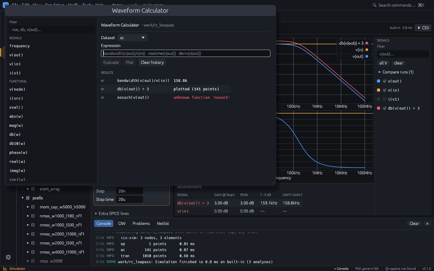
Tools > Waveform Calculator (also Simulation > Waveform Calculator) evaluates expressions on the active cell’s simulation results.
- Simulate the cell (
F5), then open the calculator. - Pick the Dataset (
op,dc,ac,tran). - Type an expression, or click a signal or a function on the left to insert it.
- Evaluate (or Enter) shows the result in Results: a number for measurements, or the point count of a waveform. Plot adds a waveform to the Simulation plot as a new signal named after the expression.
Plotted expressions are evaluated again after every simulation run, so they stay on the plot. Click an expression in Results to edit it again.
Expressions use + - * / ^, parentheses and numbers with SPICE suffixes (1n, 10k,
2meg). Signals are v(node), v(a,b) (= v(a) - v(b)), i(source) or any vector name
of the dataset (time, frequency); quote names with special characters ("v-sweep").
AC signals are complex, so v(out)/v(in) is the transfer function.
| Kind | Functions |
|---|---|
| Waveform | abs mag db db10 phase real imag conj sqrt exp ln log10 sin cos deriv integ xval() |
| Statistics | min max xmin xmax pp avg rms value(w, x) |
| Timing | cross(w, level [, n [, edge]]) delay(w1, l1, w2, l2 [, e1 [, e2]]) risetime(w [, lo%, hi%]) falltime(w [, hi%, lo%]) overshoot(w) settling(w [, pct]) |
| Frequency | bandwidth(w [, db]) ugf(w) phasemargin(w) gainmargin(w) |
edge is rise, fall or either; n < 0 counts crossings from the end. bandwidth
drops db below the first point, by default the half-power 3.0103 dB, the same point as the
f -3 dB column of the Simulation measurements (for one pole it is exactly the pole frequency). In the
Simulation plot, a real-valued result on an AC dataset (such as db(v(out))) is drawn as
it is rather than converted to dB again.
Examples on the rc_lowpass demo: bandwidth(v(out)/v(in)) is about 159 kHz;
risetime(v(out)) on tran is the 10-90 % rise time of the filtered pulse.
Corner / Sweep Manager
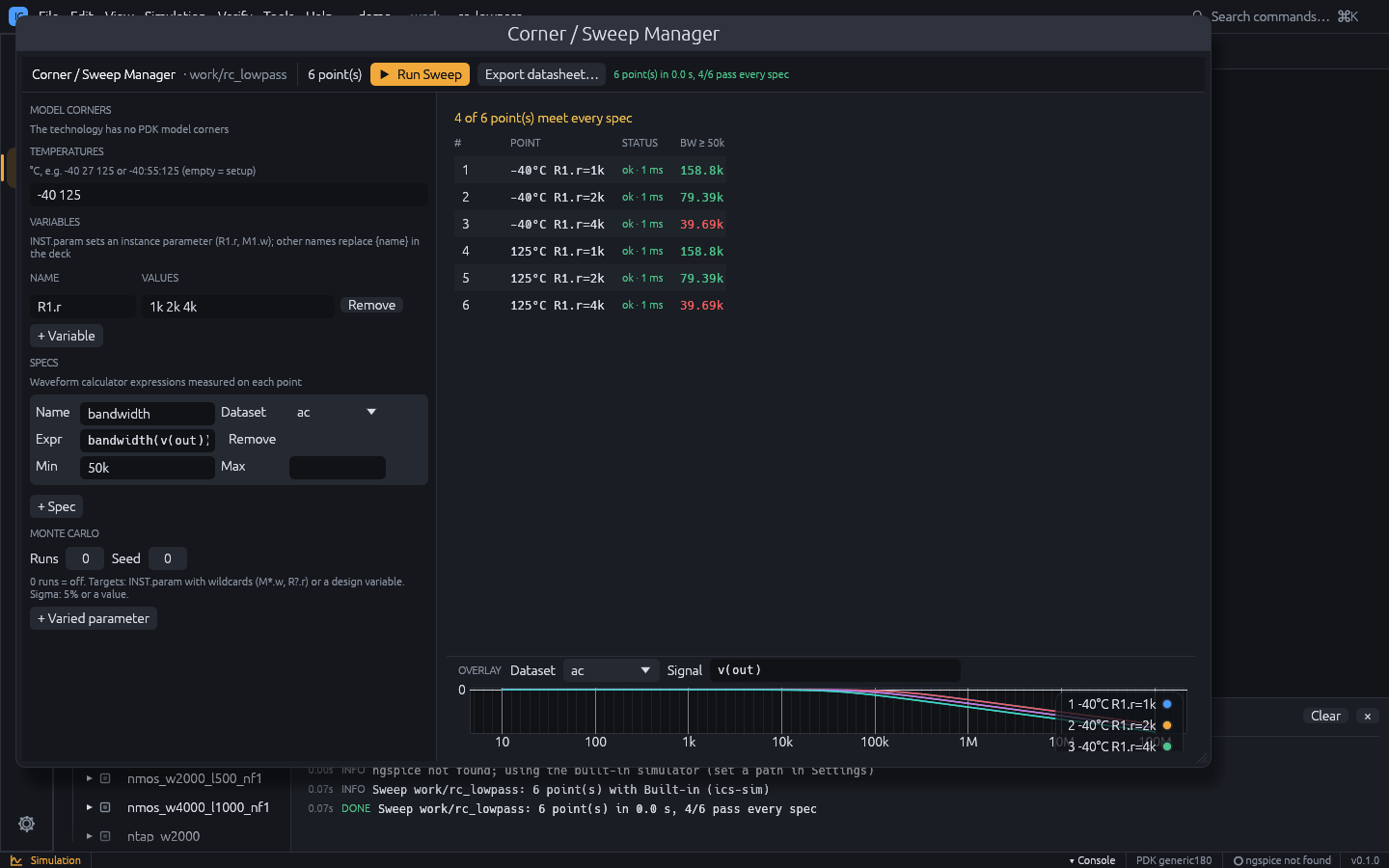
Tools > Corner / Sweep Manager runs the active cell’s simulation setup over every combination of:
- Model corners: the PDK model library’s corners (none checked = the setup’s corner);
- Temperatures: a list such as
-40 27 125or a range-40:55:125(start:step:stop); empty = the setup’s temperature; - Variables: each with a value list.
INST.paramsets an instance parameter (R1.r,M1.w); any other name is a design variable that replaces{name}in the deck, for example a source’s DC value{vdd}.
The toolbar shows the number of points (at most 2000). Run Sweep runs them in parallel on every CPU core with the setup’s backend, analyses and layout parasitics.
Specs measure each point: a name, the dataset, a calculator
expression that gives a number (bandwidth(v(out)), max(v(out))) and optional Min /
Max limits. The results table lists every point with its spec values, green when they
meet the limits and red when not, and the toolbar counts the points that meet every spec.
Overlay draws one signal or expression of every point on one plot; select a row of the
table to highlight its trace. The setup is saved with the cell (sim.json).
Monte Carlo
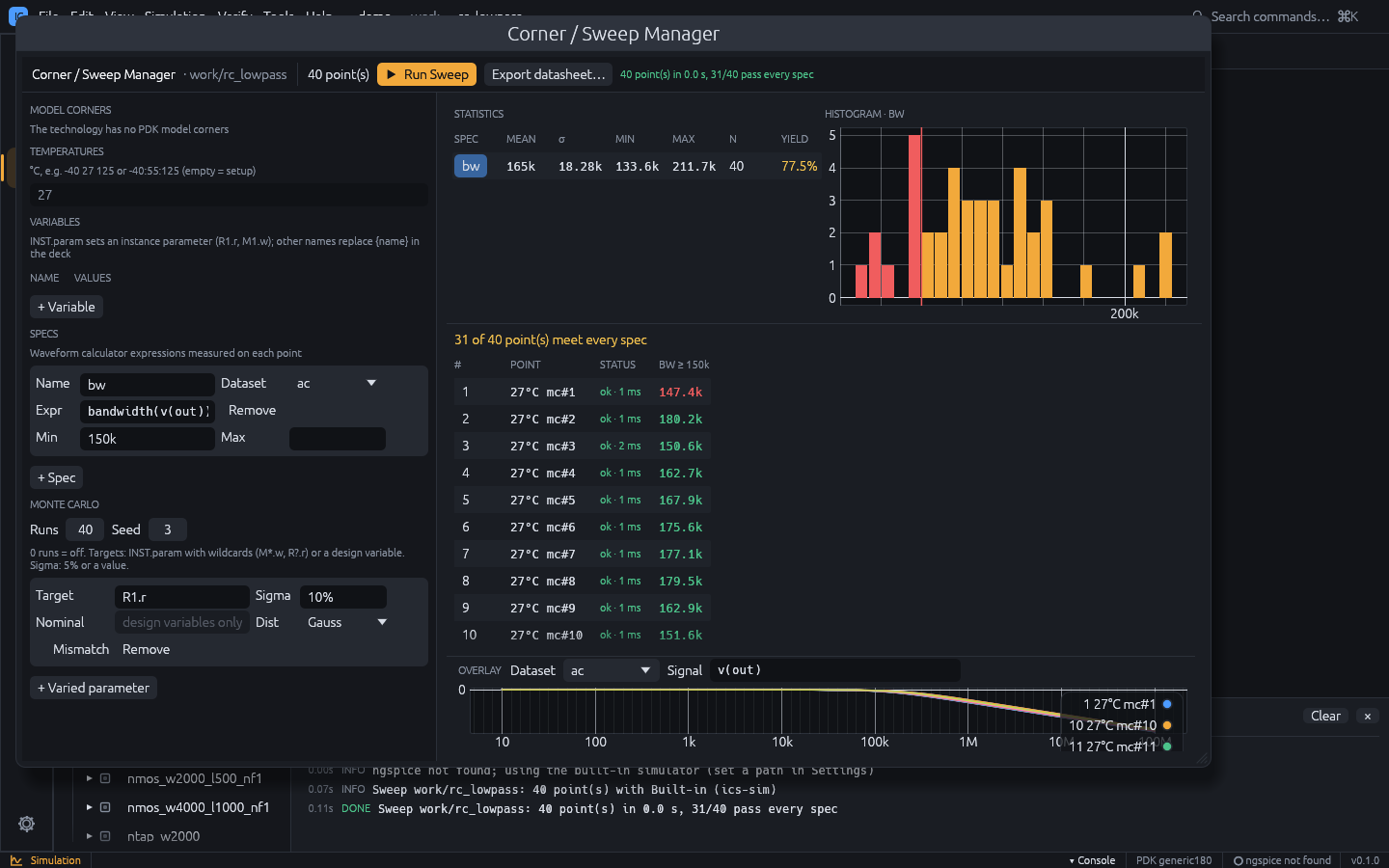
The Monte Carlo section repeats every point Runs times with random parameter values (the same samples at every corner and temperature, reproducible with Seed). Each varied parameter has:
- Target:
INST.paramwith*/?wildcards in the instance name (M*.w,R?.r), or a design variable with its Nominal value; - Sigma: a percentage of the nominal (
5%) or an absolute value; - Dist: Gauss (sigma is the standard deviation) or Uniform (sigma is the half range);
- Mismatch: draw every matching instance independently. Off, all of them share one draw per run (process variation).
With Monte Carlo results, Statistics lists mean, σ, min, max, count and yield of every spec, and a histogram of the selected spec marks the bins outside its limits in red.
Datasheet
Export datasheet… writes an HTML page of the last run: the spec summary (limits, min / mean / max / σ and yield) and the table of every point with pass / fail colours.
Optimizer
Tools > Optimizer sizes device parameters of the active cell until the specs of its Corner / Sweep Manager setup are met (at least one spec needs a Min or Max limit).
- Variables: each Target (
INST.paramsuch asM1.w, or a design variable) with Min, Max, an optional Step and Log for a log-scale search; + Variable adds one. - Evaluations: the number of candidates to simulate.
- Goal: Best margin (the largest worst-case margin to the limits) or Least area (the smallest MOS gate area once every spec passes).
- Post-layout: place, route and extract every candidate and simulate it with its parasitics, so the specs hold after layout.
Run optimizer plots the objective of every evaluation; Stop ends the run early and Apply best to schematic writes the best values into the schematic.
Results Browser
Every successful simulation keeps the previous results: the current run is Run N, and up to 12 earlier runs are listed in Tools > Results Browser and in Compare runs above the signal list of the Simulation workspace. Rename a run (for example “pre-layout”), tick it to overlay it, or Delete it.
A ticked run is drawn dashed in the colour of each plotted signal, labelled
<run>: <signal>, and gets its own rows in Measurements. A typical use is to compare
the schematic with the post-layout simulation: run once, tick Include layout
parasitics, run again and tick the first run.
Check Schematic
Tools > Check Schematic checks the active schematic; File > Check and Save does the same and saves the project when there are no errors. The findings appear in the Problems tab of the bottom panel (also kept up to date while you edit); click one to select its devices in the schematic.
| Code | Severity | Finding |
|---|---|---|
no-ground | Error | Devices but no ground |
duplicate-name, empty-name, bad-name | Error | Instance names SPICE cannot use |
missing-param, invalid-value | Error | A required value (R, C, L, W, L, model, source value) missing or not a number ({param} references are allowed) |
parallel-vsource, vsource-loop | Error | Voltage sources in parallel or in a loop |
shorted-device | Warning (Error for sources) | Both pins of a two-terminal device on one net |
unconnected-pin | Warning (Info for a MOS bulk) | A pin touching nothing |
floating-net | Warning | A net on a single pin with no label |
dangling-wire | Warning | A wire end touching nothing |
label-conflict | Warning | Two different labels on one net |
overlapping-instances | Warning | Two devices of the same kind at the same place |
isolated-net | Info | No DC path to ground |
Hierarchy Browser
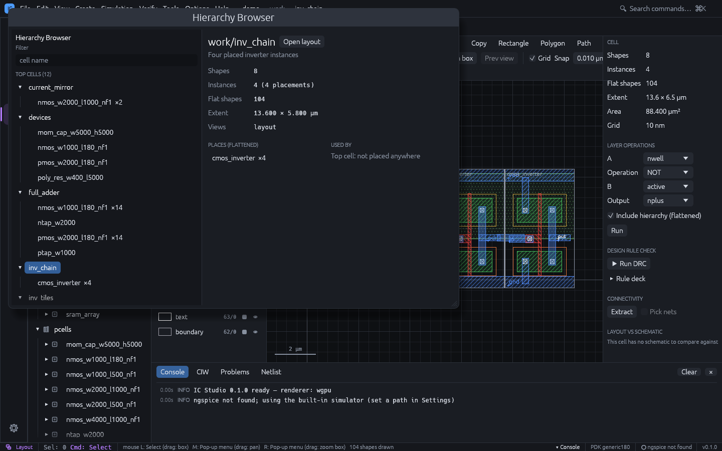
Tools > Hierarchy Browser shows every layout of the project as a tree from its top cells (layouts no other layout places), with placement counts (arrays count every element). Filter finds a cell by name.
For the selected cell it shows shapes, instances, flat shapes, extent and views, the cells
it places throughout its hierarchy with their total counts, and the cells that use it.
Open layout / Open schematic open it. The layout editor’s Hierarchy Tree
form (Edit > Hierarchy Tree, Shift+T) lists only the cells under the current cell.
Net Browser
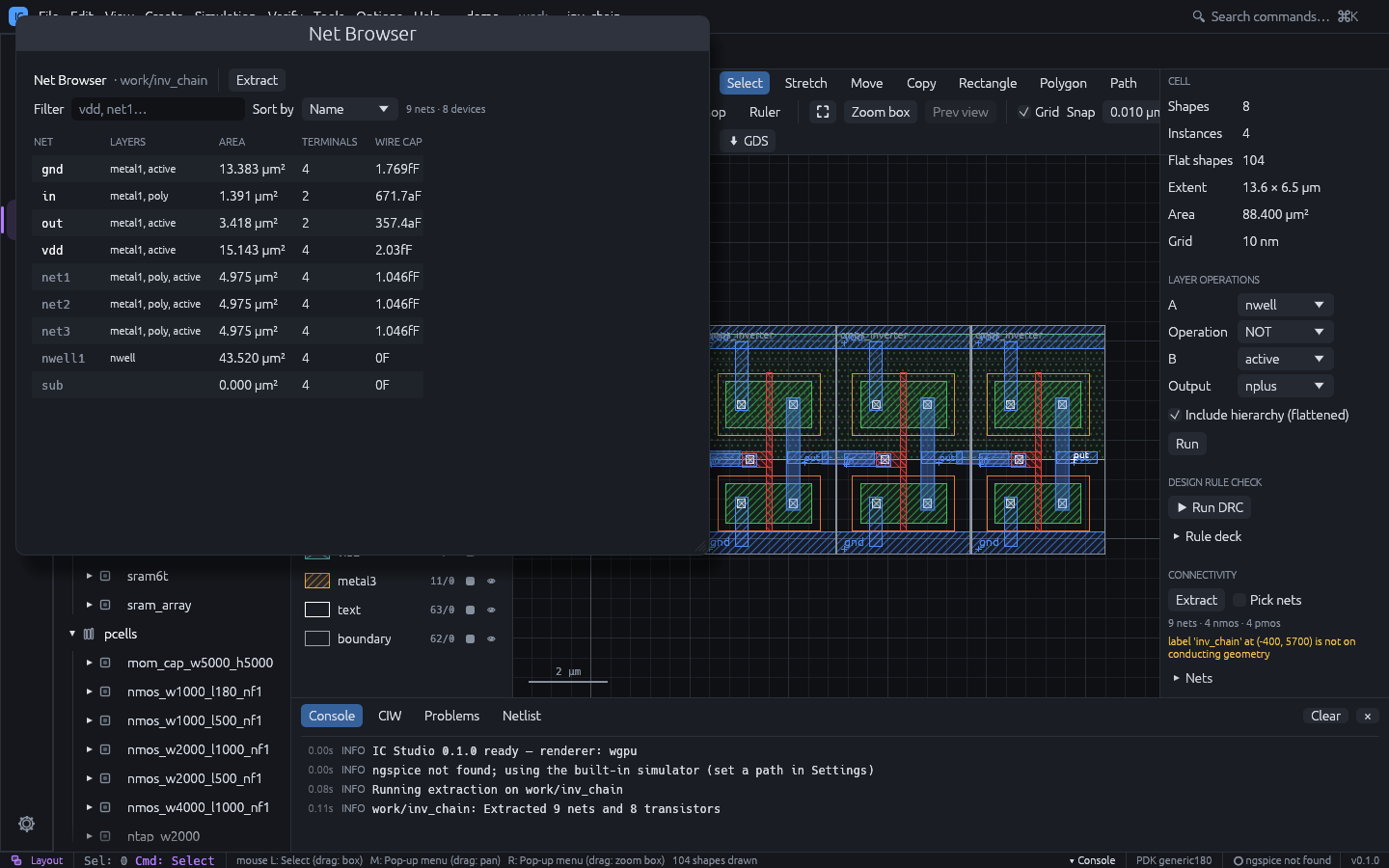
Tools > Net Browser lists the nets of the active layout’s extraction (it extracts the nets when there is no extraction yet; Extract runs it again):
| Column | Meaning |
|---|---|
| NET | Label name (bold), or a generated name for unlabelled nets |
| LAYERS | Conducting layers the net uses |
| AREA | Conductor area in µm² |
| TERMINALS | Transistor terminals (drain, gate, source, bulk) on the net |
| WIRE CAP | Capacitance to substrate from the technology’s coefficients |
Sort by name, capacitance, area or terminals. Click a net to highlight it in the layout and zoom to it. A note warns when the layout changed after the extraction.
Layout Generators
Tools > Layout Generators (Guard Ring…, Via Array…, Matched
Placement…) opens one window with four tabs. Each adds to the active layout as one step
that u / Ctrl+Z undoes.
Guard Ring
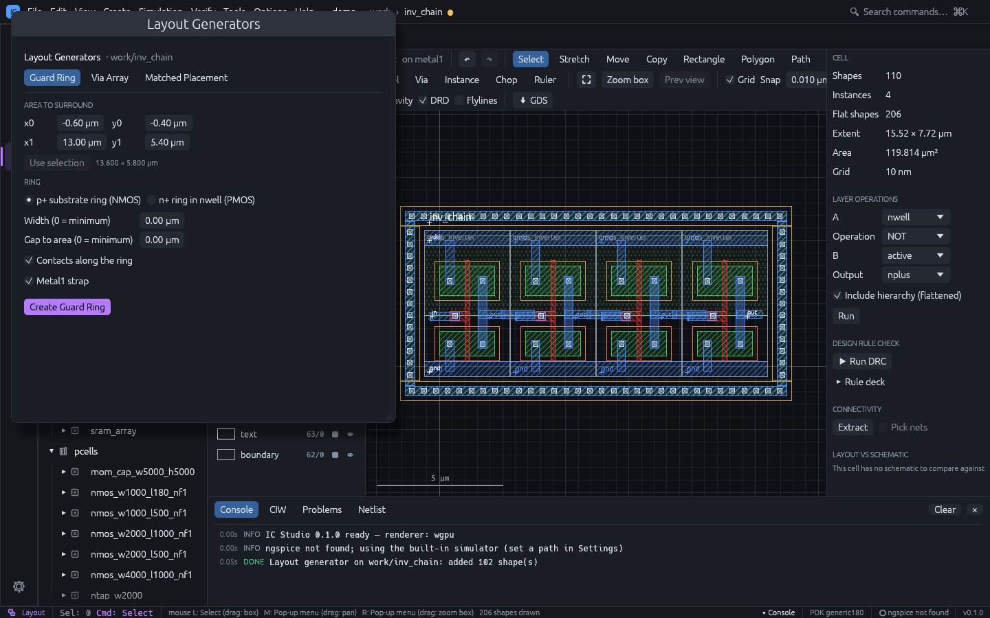
Surrounds an area with a diffusion ring: a p+ substrate ring (for NMOS) or an n+ ring in nwell (for PMOS, with an nwell covering the ring and the area). The ring has its implant, optional Contacts along every side and an optional Metal1 strap. Width and Gap to area of 0 use the minimum from the layer and contact rules. Set the area in µm, or press Use selection to take the bounding box of the selected shapes and instances. With contacts and the strap, the ring is DRC clean on its own.
Via Array
Pick a via, then either:
- Every overlap of the via’s layers: a via array in each overlap of its bottom and top layers (through the hierarchy), optionally only within the area; or
- Fill the area: as many cuts as fit, centred, with enclosing pads on both layers.
Cut size, spacing and enclosure come from the via definition.
Matched Placement
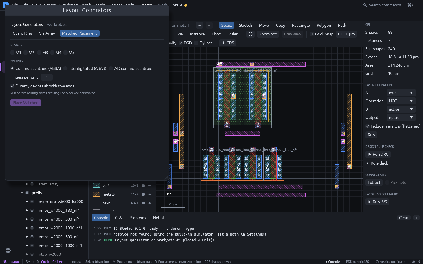
Re-places matched MOS devices of the layout (for example a differential pair or a current mirror) as unit devices in a pattern:
| Pattern | Example |
|---|---|
| Common centroid | A B B A, one row, mirror-symmetric |
| Interdigitated | A B A B |
| 2-D common centroid | A B / B A, Rows rows, point-symmetric |
Tick the devices, set Fingers per unit and whether to add dummy devices at both
row ends. The devices must have the same type, L and finger width, and every device’s
fingers must be a multiple of the unit. Each device keeps its total W; its units are named
<device>.<k>, so flylines, routing and LVS still map them to the schematic device (LVS
merges the parallel units). Dummies have gate, source and drain tied to the bulk net and
are dropped by LVS. Neighbouring devices are moved aside to make room.
Run it before routing: wires crossing the block are not moved. Common centroid allows at most one device with an odd number of units; with single-finger devices use interdigitated, or more fingers per device.
By Example
Reuses the placement of a finished cell with the same circuit. Pick the Reference (a cell with a schematic and a placed layout) and press Place like reference: devices are matched by topology, placed where their counterparts are and sized from this cell’s schematic. Wells, implants and taps are copied; wires are not, so tick Route the flylines afterwards to route them again.
DRC Rule Designer
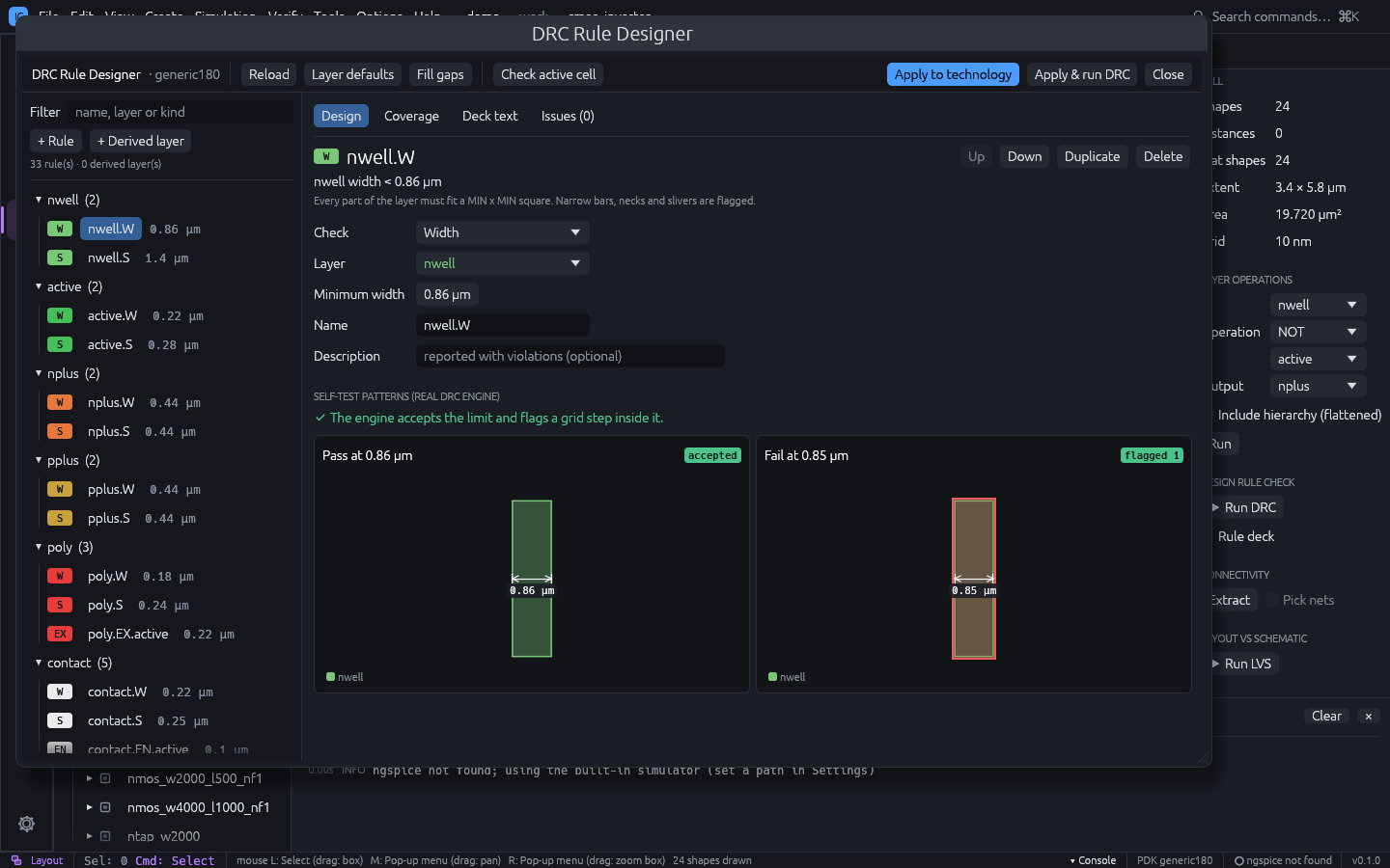
Tools > DRC Rule Designer (also Rule Designer… in the Rule deck section of the layout inspector) edits the technology’s DRC deck as forms instead of text.
- Start here: a step-by-step guide for people new to DRC (start from a deck, fill the gaps, fix problems, add rules, try the deck on the active cell, apply), a glossary and a picture of every kind of check.
- Rule list (left): rules grouped by layer with their values; + Rule opens a gallery of checks drawn as pictures with the question each answers, marking the ones recommended for the chosen layer; + Derived layer offers presets (transistor gates, poly outside active, wide metal) or a custom expression; Filter finds a rule.
- Design: the selected rule’s check, layers, value, name and description, with the technology’s value next to the field and a Use button when they differ. Every rule is self-tested on generated pass and fail patterns with the real DRC engine, drawn side by side, so you see that the engine accepts the limit and flags a violation one grid step inside it.
- Coverage: a matrix of which checks each layer has.
- Deck text: the generated deck.
- Issues: lint findings, such as duplicate rule names, rules that can never fire, values off the manufacturing grid, unused derived layers and routing layers without a width or space rule. Most come with a one-click fix (snap to the grid, rename, remove a redundant rule, add the missing rule); Fix automatically applies all fixes of errors and warnings and adds the missing rules.
The toolbar has Reload (the technology’s deck), Layer defaults (the deck derived from the layer and via rules), Fill gaps (adds missing width / space rules of routing layers and via enclosures with technology values), Check active cell (runs the draft deck and counts violations per rule), Apply to technology and Apply & run DRC.
Stream Layer Map
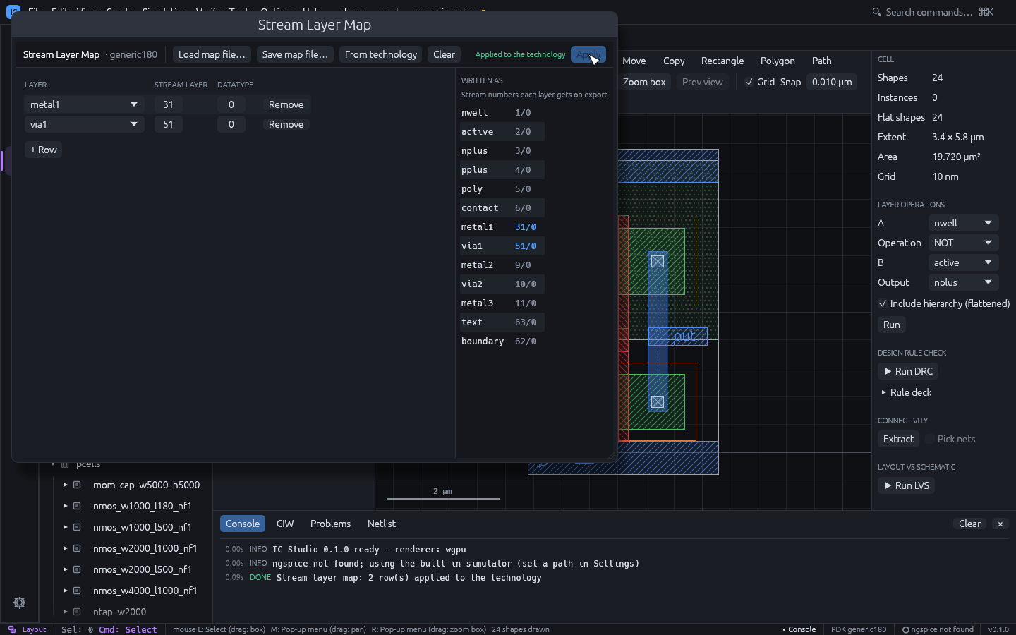
Tools > Stream Layer Map sets which GDSII / OASIS layer and datatype each technology layer is written as and read from, like a Virtuoso XStream layer map. Each row maps a stream layer / datatype to a technology layer:
- on export, a layer is written with the numbers of its first row (layers without a row keep their own numbers; Written as previews the result);
- on import, shapes on the row’s numbers go to that layer, so several stream numbers can map to one layer; (drop on import) discards them.
Load map file… reads a Virtuoso layer map (layerName purpose streamLayer streamDatatype per line, # comments); a purpose other than drawing names the layer
name.purpose, namepurpose or name_purpose. Save map file… writes one, From
technology starts with one row per layer, Clear removes the map. Problems (unknown
layers, a number pair mapped twice, two layers written as the same numbers) are listed
above the table. Apply stores the map in tech.json (stream_map).
The map applies to File > Import / Export, ics gds, ics import-gds and the MCP
import_gds / export_gds tools. The project’s own library files are not affected.
Dummy Fill
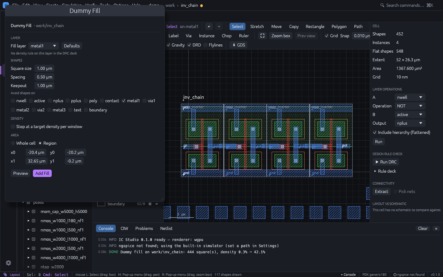
Tools > Dummy Fill adds grid-aligned fill squares to a layer, to meet a density rule.
- Pick the Fill layer. The defaults come from its rules: squares of four times the min width (at least 1 µm), spacing twice the min spacing, keepout of at least 1 µm, and the window, step and a target just above the minimum of the deck’s density rule on the layer, if there is one.
- Set Square size, Spacing, Keepout and the layers to Avoid (fill keeps the keepout from their shapes, through the hierarchy).
- Optionally tick Stop at a target density per window: each window is filled only up to the target, and never above the rule’s maximum.
- Fill the Whole cell (its bounding box) or a Region in µm.
- Preview shows the square count, the density before and after, and whether every window passes the rule; Add Fill adds the squares (undoable).
A compact cell may have no room for fill inside its bounding box; fill a larger region around it instead.